
Chapter 1: The Scientific Method


Figure 1. Deductive and inductive reasoning in the scientific method. Making sense of the natural world begins with observations. Left) As we collect observations of the world, we can begin to make general predictions (or perceptions) regarding phenomena. This process is known as inductive reasoning, making general predictions from specific phenomena. From these generalized perceptions of reality, specific predictions can be deduced using logic, generating hypotheses. Middle) Experimentation allows researchers to test the predictions of the hypotheses. If a hypothesis is falsified, that is another observation which adds to our general perception of reality. Right) As more and more similar but different experiments reinforce a specific prediction, growing support emerges for the development of a scientific theory, another example of inductive reasoning. In turn, a theory can assist in the development of additional, untested hypotheses using deductive reasoning.
The scientific method was developed in the 17th century as a method of inquiry to acquire new knowledge or modifying our existing understanding of natural phenomena through process of observation and experimentation. Empiricism is a core principle of scientific method, which maintains that true knowledge is best achieved through sensory experience. This method of inquiry allows measurable results from experimentation to be analyzed with predicted results, generated through observations of the natural world. While the details of the scientific method vary among the disciplines, the basic framework consists of observations resulting in the development of hypotheses, experimentation, measurements to test hypotheses, and an analysis of results to support, reject or help modify the hypotheses.
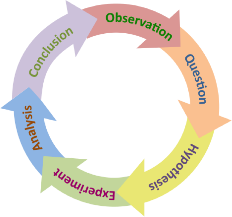
Figure 2. The Scientific Method. Observations of the natural world lead to questions. Scientific questions generate hypotheses, many of which may be tested through controlled experimentation. Experimentation and analysis allows hypotheses to be falsified, which provide information (or conclusions). The process of scientific experimentation leads to more observations and questions.
Deductive and Inductive Reasoning
Science is an interplay between deductive and inductive reasoning (fig. 1). Experimentation is principally based on deductive reasoning, which starts out with a general understanding of a phenomenon and examines known possibilities (or hypotheses) using rules of logic to eliminate (or deduce) false truths to arrive at a specific conclusion. A biological example would be: "All humans are animals. All animals are eukaryotes. All eukaryotes have cells containing a nucleus. Therefore, all human cells have a nucleus." Inductive reasoning is a principle of logic directly opposite of deductive reasoning. Specific phenomena infer general predictions. In our previous example: "All human cells have a nucleus. All eukaryotes have cells containing a nucleus. All animals are eukaryotes. Therefore, all humans are animals." While science is primarily based on deductive reasoning, inductive reasoning does have its place. Observations of nature are specific in nature. As observations of a specific phenomenon amass, a researcher begins to emerge with a general understanding of that phenomenon (inductive inference), which in turn results in the development of specific hypotheses. Once hypotheses are established, experimentation produces results to reject false hypotheses and support unfalsified hypotheses. As a collection of unfalsified hypotheses get researchers closer and closer to 'the truth', inductive reasoning can be used to develop a scientific theory, which explain and make accurate predictions in a wide range of circumstances.
Developing a Scientific Question
Observations of nature allows humans to generate a variety of questions (inductive reasoning), some of which can be answered scientifically. A scientific question is: simple, measurable, testable, answerable, and specific in scope. Perhaps one of the great powers of science is simplicity of the questions asked. Testing simple questions provide incremental knowledge, which build upon one another eventually allowing a grander, more accurate, understanding of natural phenomena. Typically, scientific questions have yes/no answers; either there is an effect or there isn't. The best experiments stemming from scientific are typically quite specific in scope: "Does x cause y?" A controlled experiment is the gold standard of the scientific method, in which a single variable is changed and the effect is measured. As the effects of individual variables are understood, scientists seek to understand more complex interactions. However, increasing complexity increases uncertainty, and typically reduces predictive power. As a the interactions of a complex scientific phenomenon becomes better understood from the analysis of many related, but simpler questions, a scientific theory may emerge.
Hypothesis: more than an educated guess
A hypothesis is a testable explanation for an observable phenomenon. Hypotheses are generated based on previous observations of nature that can not be explained by existing hypotheses or theories, and must be testable and falsifiable. The purpose of testing hypotheses by experimentation is not to prove a hypothesis, but to disprove inaccurate hypotheses.
Experimentation and data analysis allows scientists to determine whether the hypothesis is a potentially valid explanation of a natural phenomenon or not. In this way, science is revealing the reality of nature by removing falsified hypotheses. In other words, science reveals 'nature' by removing what is 'not-nature'. Hypothesis testing must be observable and repeatable. In this manner, independent research may revisit and retest the hypotheses. Hypotheses may be supported in one experiment, but rejected in separate experiments. When this happens, further experimental repetitions may need to be conducted to analyze the validity of the hypothesis.

Figure 3. Null and alternative hypotheses. Every experiment simultaneously tests several hypotheses. In an experiment analyzing the effects between two phenomena, the null hypothesis is there is no difference between those phenomena. An alternative hypothesis states that there is a difference between the phenomena. Different alternative hypotheses will include (1) x is not equal to y, (2) x is greater than y, and (3) x is less than y.
Every experiment tests multiple hypotheses simultaneously (fig. 3). A null hypothesis (H0) states that there is no relationship between two phenomenon. An example of a null hypothesis is, "H0: There will be no relationship between chemical reaction rates." If the null model is rejected, this infers there is a potential relationship between these phenomenon. In this case, one or more alternative hypotheses (HA) can be proposed to explain the relationship between measured phenomena. Two alternative hypotheses for the proposed null hypothesis are: "HA1: As temperature increases, chemical reaction rates decrease." and "HA2: As temperature increases, chemical reaction rates increase." In this example, the alternative hypotheses infer that temperature causes a change in chemical reaction rates. While this may be true, a scientist must be careful to separate correlation from causation.
Correlation is not causation, or is it?
Pure causation indicates that x causes y. In our example, an inference of pure causation would be, "Higher temperature causes an increase in chemical reaction rates." This statement is typically true in chemistry. Heating a solution allows chemical reaction to occur more rapidly. Pure causation is typically inferred in many scientific studies, however a scientist should always consider the many different mechanisms that two variables are correlated.

Figure 4. Possible relationships between correlated phenomena. Direct causation: x causes y. Reverse causation: y causes x. Common causation: z affects both x and y. Cyclic causation: x affects y, and y affects x. Indirect causation: x affects y, but indirectly through another variable, z. Coincidence: x and y are related, but there are no known causal relationships.
The opposite of pure causation, known as reverse causation, is where a correlation is present because y causes x. An inference of reverse causation in our example would be, "Higher chemical reaction rates increase temperature." If you have used hand warmers, those little plastic bags you break open and heat is generated, you have experienced the effect of chemical reactions generating heat.
A third possibility is common causation, where x and y are both affected by a third variable. A classic example is that ice cream sales and drowning deaths are positively correlated. We know ice cream sales don't cause drownings. Rather there is a third variable (temperature) that is positively associated with both variables: ice cream and drownings.
Cyclic causation occurs when there is a feedback between the variables under consideration. A classic biological example is the numbers of predators and prey are dependent upon each other. If predators increase, prey decrease. If prey increase, predators increase. If prey decrease, prey decrease. Deconstructing these relationships is often very difficult.
Indirect causation happens, when x is correlated with y, but the effect on y is directly affected by another variable, z, which in turn is affected by x. Indirect causation is very commonly found in community ecology. Suppose a researcher is concerned about a predator on the endangered species list. Considering just the numbers of prey is too simplistic of an approach to adequately model predator population. Revisiting the predator/prey relationship, consider a third variable: plant biomass. Prey abundance is correlated with plant abundance. Therefore, predator abundance (y) can be predicted by calculating plant biomass (x), which directly affects prey abundance (z). In other words, plant biomass directly affects prey abundance, which directly affects predator abundance. Predator abundance is indirectly correlated to plant biomass.

Figure 5. Correlation between rates of autism and organic food sales. These variables are highly correlated, but clearly organic food sales are not responsible for increasing autism rates.
Occasionally, two variables are correlated simply by coincidence. In any given random statistical comparison, variables will correlate with each other 5% of the time when the confidence interval is at 95%. This is a primary reason that repeating experiments is so important. While it is not uncommon to find correlations between random variables, additional investigations will be able to examine the validity of actual correlation. If many experiments show a correlation between unsuspecting variables, evidence emerges that a real correlation exists. For example, increasing autism rates in the US are positively correlated with organic food sales. Clearly, there is no causation of organic food on autism. More likely, the detection of autism has refined at the same time as an increasing desire for people to eat organic food. It is purely coincidental.
Proving causality has proven much more challenging than measuring correlation. Much has been written on the topic of causality from the philosophers of ancient Greece to contemporary physicists studying the butterfly effect, a nonlinear feedback system where the smallest changes in the inputs can result in drastic changes in the output. Many philosophers, statisticians and even scientists suggest that it is impossible to prove causality of any effect. We can only infer correlation. While this is true, a well-designed experiment seeks to minimize this uncertainty.
A well-designed experiment
The purpose of the experiment is to provide insight into causation by manipulating an experimental variable (or variables), in order to validate or reject competing hypotheses. While the scope and scale of experiments vary widely within science, well-designed scientific experiments have certain characteristics:
- An experiment must be repeatable. An experiment that is not repeatable can not be verified, and therefore is simply an observation. An experimental discovery that is reproducible provides high precision between expected and observed results, which in turn supports consensus on the effect.
- An experiment contains many replicates. Making a single observation of a phenomenon is not an experiment, but an observation. Hypothesis testing is conducting using statistics, which requires replicates. A replicate is the repetition of an experimental condition on different subjects (or units, more generally), in order to measure and account the variability within the groups examined. Furthermore, statistics assumes replicates are representative of the population being studied, and preferably randomly selected.
- An experiment imposes a treatment and assesses the effect. A treatment (also called the experimental variable) is the variable that scientists alter within an experiment. For example, if a study was comparing the effect of sugar consumption on exam scores, the experimental variable would be the sugar. It is the component of the experiment that will differ between the groups. Replicates are assigned to a control group and one or more experimental groups, and the effect of the treatment is assessed. The control group is a random subset of the subjects (or units) to be examined that either do not receive the treatment, or receive the standard treatment. In our example above, it may not be advisable for a group of students to receive no sugar. In this case, they would receive the minimal dosage necessary. An experimental group (or treatment group) receives the experimental treatment. There typically may be several experimental groups, each receiving varying amounts of the treatment, in order to assess the effect of the treatment at different levels. Control groups provide a baseline to compare the change in the experimental groups based on the effect of the treatment.
- Ideally, all variables in an experiment are kept constant except the treatment. While this is not always possible, it is the gold standard of experimental design. If an effect of the treatment is found under such circumstances, much more weight is given toward the direct causation of the treatment.
Types of experiments
Controlled experiments
Ideally, scientists conduct a controlled experiment, in which two (or more) groups (or samples) are established, and receive exactly the same treatment except for the alteration of a single variable, the experimental variable. Typically one of the groups, known as the control group, will not have the experimental variable (or receive a placebo – a substance known to have no effect). A group that receives the experimental variable are known as the experimental group. More than one experimental group is generated when a scientist wishes to determine the range of effects of the experimental variable at different concentrations. By constraining all parameters in the control and experimental group(s), but only changing a single parameter (the experimental variable), any measured variation between the groups can be inferred to be a function of the experimental variable.
Drug trials are classic examples of a controlled experiment. The group of subjects receiving the drug are within an experimental group. Typically, varying dosages of the drug are administered to different experimental groups. Subjects not receiving the drug represent the control group. Typically, subjects within the control group receive a placebo, a simulated or ineffectual treatment. Drug trials are typically run as blind experiments in which the replicates are not aware if they are receiving the actual treatment (drug) or a placebo. In a double-blind study, the experimenters are kept in the dark as well, in order to minimize researcher bias. Interestingly, many subjects within the control group in a double-blind study of drug trials achieve a measurable response (either positive or negative) from the placebo, known as the placebo effect. To measure the placebo effect, an additional control group (known as a negative control) may be assessed, in which they receive no treatment whatsoever. A positive control is a known effect from the experimental treatment, used to confirm to validity of the measurements acquired. A negative control should provide support to the null hypothesis, indicating no effect between the measured phenomena. Often, negative controls can also be used to establish a baseline result, or to subtract a background value from the test sample results.

Figure 6. Dependent vs. independent variables. This is a useful tool for determining the dependent and independent variables in an experiment. Once you identify the variables in an experiment, plug them into: ___ depends ___. The first word will be the dependent variable and the last will be the independent variable. Dependent variables are the manipulated variables (or inputs) within a controlled experiment, whereas the independent variable is the expected effect (or output).
In a controlled experiment, the variable in which the inputs are purposefully manipulated is the independent variable, whereas the variable expected to change (output) based on the presence or abundance of the experimental treatment is the dependent variable. Variables that are kept constant for the control and experimental groups is known as a control variable. For example, in a study that is measuring the effect rabbit abundance in the the presence or absence of wolves, the independent variable would be the presence or absence of wolves. In this example the measured effect (or dependent variable) is the abundance of the rabbit population. Many students struggle to differentiate between independent and dependent variables. The easiest way is to complete the statement (fig. 6), " ___ depends on ___." In our example, "The abundance of rabbits depends on the presence or absence of wolves." If you complete the sentence and it makes sense, the former is dependent variable while the latter is the independent variable. Another way to think about it is what is the variable you are controlling (independent variable) and which one are you expecting a response from the input (dependent variable).
Natural Experiments
Controlled experiment are sometimes prohibitive to impossible. Consider a researcher analyzing the effect of rainfall on bird diversity in tropical islands. Rainfall cannot be controlled at such a large scale as is required in a controlled experiment, leading the researcher to employ a natural experiment. Natural experiments are considered quasi-experiments, as the manipulation of variables are outside the researcher's control. In a natural experiment, researchers rely on observations of replicates exposed to a variety experimental and control conditions, and infer an effect. The experimental design of natural experiments seeks to select replicates that closely resemble each other as possible, but vary in preferably one factor. In our example, a researcher would select tropical islands of approximately the same size, structure and composition as is possible, but are known to vary in precipitation amounts. Through careful selection of replicates, effects of the independent variable (i.e. rainfall) on the dependent variable (i.e. bird diversity) can be analyzed. Obviously, it is impossible to select islands that are exactly the same in every way. There will always be variation in island size, distance from other islands, plant diversity, topography, and many other factors. Often known variabilities are also included in a more complex statistical model to determine how all of these factors interact. However as these models increase in complexity, their predictive power diminishes exponentially. Determining causation from correlation from natural experiments is challenging at best.

Figure 7. Correlation between average global temperature and atmospheric carbon dioxide. Analysis of global warming is a natural experiment. While carbon dioxide and global temperatures are highly correlated, and increasing since the mid-1800s, additional controlled experiments are useful in supporting a case for causation.
Perhaps, the largest scientific controversy of modern times is climate change. The earth is warming, an indisputable fact. The cause of global warming has been a source of contentious debate among scientists and politicians for decades. The root of this controversy is due to the fact analyzing the causal factors of warming at a global scale is conducted as a natural experiment or mathematical model, as we don't have several replicate earth-like planets to control. With that said, presently no national or international scientific organization disagrees with the hypothesis that global warming is human-caused. Moreover, nearly all scientists agree greenhouse gases are the culprit. Ever since the birth of the industrial revolution, humans have been releasing greenhouse gases into the atmosphere at increasing rates. Average global temperature is highly correlated with atmospheric carbon dioxide (fig. 7). At face value this is simply an observation, that doesn't imply causation. Smaller scale controlled experiments can help assist researchers to determine causation. For example, an experimental design including groups of replicate 'atmospheres' in sealed containers with varying amounts of carbon dioxide could be exposed to the same amount of light energy. Any discrepancy in temperatures between the replicates could be attributed to the abundance of carbon dioxide. In this manner, natural experiments serve as observational studies in which larger scale hypotheses can be generated via inductive reasoning. Smaller scale controlled experiments test these assumptions using deductive reasoning and controlled experimentation and hypothesis testing. If observations of these different approaches are equitable, then there is a stronger support for a causal effect.

Figure 8. Descriptive statistics describe the central tendency and variability of data. The mean (μ), is the measure of the observed average numerical value of a population of data, whereas the standard deviation (σ) is a measure of the variability of a population of data. If data are normally distributed, the first deviation represents 68% of the observations, while the second and third deviations represent 95% and the 99.7% of the observations.
Data analysis
Descriptive statistics define observations
Descriptive statistics summarize two aspects regarding the distribution of data: central tendency and variability (fig. 8). Central tendency is a measure of the distribution's central (or most common) value. The mean of observed data, known as the sample mean (x̅), represents the mathematical average of the data and is calculated as the sum of observations (Σx) divided by the number of observations, known as the sample size (n): x̅ = Σx / n. Where the mean is the calculated middle of the data, the median represents the observed value of the middle. For example, in the data set [1, 2, 3, 6, 7, 7, 9], the median is 6, the middle number in the ordered observations. If there are an even numbers of observations, the middle two observations are averaged. Occasionally a researcher is interested in most common value, or mode, rather estimating the middle. In the previous data set the mode is 7. Analyzing the distribution of the data is necessary to determine the appropriate measure of central tendency. A mean is typically used when there is a large sample size and few outliers (extreme observations). Hypothesis testing of means typically assumes a normal distribution of data, commonly known as the bell shaped curve, in which most observations are made surrounding the central value and become increasingly less frequent further from the center. When data are not normally distributed, the median is considered a better representation of the typical value. For example, analyses of income typically examine the median, as income is typically skewed due to the presence of extremely high and low income values.

Figure 9. Visualization of how standard deviation (σ) is calculated. Standard deviation (σ) is a cumulative measure of the deviations of observed values (xi) and the sample mean (x̅). To calculate standard deviation, take the square root (√) of the sum (∑) of squared deviations of the sample mean (x̅) from the observed value (xi), divided by the sample size minus one (n-1).
Variability is a measured deviation of data from the central tendency, and is also calculated in a variety of ways. The most common measure of variability is standard deviation (σ). A low standard deviation indicates a small variation in the data from the mean, where a high standard deviation indicates data are spread across a large range of values. The standard deviation is commonly used as a measure of statistical confidence. Low standard deviation indicates a high confidence that the measured sample represents the population as a whole. For example, if you measured the height of several random people would that represent the variability in height for the whole human race? Standard deviation is inversely proportional to the sample size. More measurements of height provide a smaller standard deviation. Scientific experiments ideally have many replicates to minimize the effect on standard deviation based on small sample sizes. If the standard deviation is acceptably low, this tells us that the sample mean is very close to the population mean.
Descriptive statistics are useful in identifying typical observations and detecting extreme observations. For example, the mean (μ) height of adult men is 178cm with a standard deviation (σ) of 8cm. Interpreting the mean alongside the standard deviation suggests most adult men (68%) will be 178±8cm tall, between 170 and 186cm. Two standard deviations (2σ) account for 95% of the variation, also known as the 95% confidence interval. So 95% of adult men are between 178±16cm tall, or the 95% confidence interval for human male adult height is between 162cm and 194cm. Three standard deviations (3σ) account for 99.7% of the variation in the data. Nearly all adult men (99.7% to be precise) are predicted to be between 146cm and 202cm.
Inferential statistics test hypotheses
While descriptive statistics describes the nature of sampled observations, inferential statistics infer predictions of the larger population that the sample is based on. Experiments produce data, which in turn are used to conduct hypothesis testing to determine the probability of competing hypotheses. Hypothesis testing is a statistical inference that measures the relationships between the control and the experimental groups. The predictions of each hypothesis are compared to the observed phenomena and typically examined with statistical analysis. If the observed phenomena violate the predictions of the hypothesis, the hypothesis is said to be rejected. If observations do not violate the predictions of the hypothesis, the hypothesis is said to be supported. In this case, some scientists prefer the terminology “fail to be rejected” in lieu of supporting a hypothesis. The reasoning behind this is that even though a hypothesis is supported in one experiment, it can be invalidated in further investigations. The main function of experimentation is the falsification of hypotheses (or disproving hypotheses), not proving hypotheses. In this manner, scientists are not revealing nature, but exposing nature by revealing “not nature.” If a difference between the groups is not found, the null model is supported indicating no relationship between the groups, and therefore no effect of the experimental treatment. If hypothesis testing detects a difference between the data sets, this infers that the experimental treatment has produced some effect on the dependent variable, supporting one of the alternative hypotheses. Additional analysis is conducted to quantify the effect, which can be used to make predictions for future experiments.
To test the competing hypotheses, a researcher must identify a statistical test appropriate for the experimental design. There are many statistical tests, which differ in their assumptions about the data being compared. Are the data continuous (i.e. time) or categorical (i.e. male v. female)? Are you comparing relationships between dependent (i.e. rabbit abundance) and independent variables (i.e. presence or absence of wolves), or comparing different groups (i.e. olympic medal counts of different countries). Are the data normally distributed? Are there equal variances between groups?
Figure 10. Decision tree for hypothesis testing using Student's t-test. The p-value of a t-test determines if there is a significant difference the sample means between the control and experimental groups. If p ≥ 0.05, there is no statistical difference, supporting the null hypothesis indicating no effect of the treatment on the dependent variable. If p < 0.05, the null hypothesis is rejected, indicating some effect of the treatment on the dependent variable. If the sample mean (x̅) for the control group is larger than the sample mean for the experimental group, the alternative hypothesis suggesting the treatment decreases the dependent variable is supported. Alternatively, is the mean of the experimental group is higher, it is concluded the treatment increased the dependent variable.
Once an appropriate statistical test is selected, descriptive statistics help researchers identify a relevant test statistic (e.g. mean, median or some measure of variance between the groups). The observed values are used to calculate the test statistic, which is then compared with the expected values of the test statistic under the null hypothesis, by calculating the p-value. The p-value allows us to determine whether or not the test statistics (e.g. means) of the two samples differ “significantly”. When you take a statistics class, you will learn how this statistic is created. For our purposes, it is sufficient to be able to interpret this statistic without calculating it. The p-value is the probability (ranging from zero to one), that infers whether or not the observed test statistics (e.g. means) of two samples are likely to be different and not merely a product of chance. In most biological studies, if the p-value is less that 0.05 we can state that there is, in fact, a “statistical” difference between the two populations. This is a somewhat artificial cut off, but it is one that is widely accepted in this field of study. The smaller the p-value is the stronger the evidence against the null hypothesis and the higher likelihood that the test statistics actually differ, and increasing support for one of the alternative hypotheses.
Let's see an example by testing the null hypothesis:
H0: There is no difference between maze completion times in mice that receive water and mice that receive coffee.
In this experiment, mice would be selected and placed into the two groups: one group given water and the other given coffee. Mice would be allowed to complete an unknown maze with a food treat at the end, with the observations being measured completion times. To test this hypothesis we would conduct an unpaired t-test, which compares the means of two data sets which are not directly related. Mouse A that receives water has no effect on mouse B that receives coffee. Conducting a unpaired t-test allows the researcher to compare the variation (standard deviation) along with the mean to support or reject the null hypothesis by predicting whether or not the observed means differ from each other significantly. While the process of calculating p-value is beyond the scope of this exercise, we can still interpret it.
If a different experiment were conducted examining maze memorization rates on the two groups, the researcher would compare the difference between in maze times from the first and second run through of the maze of the same mouse (Δtime) with the observation being the first time subtracted from the second time (Δtime). For this test the researcher would conduct a paired t-test, which compares the means of two observations known to be related. In our example, the first and second maze completion times are expected to be correlated because the same mouse is performing. If a difference was found between Δtime in both groups, then a second statistical test could be used to detect a difference in Δtime between mice that received water and those that received coffee.
If the results from the experiment support a hypothesis, confidence in the validity of the hypotheses enhances, but does not “prove” the hypothesis is actually true. Future experiments may reveal contrary results. For example, if a hypothesis is rejected during one experiment, it may be supported in a subsequent experiment (or vice versa). If the experiment is repeated a large number of times with same result, the hypothesis may be validated by the larger scientific community. Yet, scientific hypotheses are never said to be “proven,” because new data or alternative hypotheses may emerge to disprove previously supported hypotheses.

Figure 11. Pasteur's experiment testing spontaneous generation and biogenesis. Pasteur invented the swan-necked flask to create an environment known not to grow microorganisms. After sterilizing a nutrient broth in these flasks, he removed the swan necks of the samples in the control group. Microorganisms grew in the control group, but not the experimental group, supporting biogenesis and rejecting spontaneous generation.
Pasteur's experiment testing spontaneous generation
Louis Pasteur is best known for his research with microorganisms and invention of process that bears his name, pasteurization, in which liquids such as milk or beer heated to a temperature between 60˚ and 100˚C killed many of the microorganisms that spoiled these liquids. Once pasteurized and sealed, the liquids would no longer spoil. This discovery drove Pasteur to disagree with a commonly held theory of his day, spontaneous generation
Spontaneous generation predicts that living organisms emerge from non-living matter. Fleas arise from dust or maggots emerge from flesh, all spontaneously without any living organisms interference. The theory sounds ridiculous to us today, but during Pasteur's time it was widely regarded as fact, with a long history (over two millennia) dating back to Aristotle and beyond. Old ideas are hard to change.
In his development of the process of pasteurization, Pasteur began to disbelieve spontaneous generation in lieu of an alternative hypothesis, biogenesis, hypothesizing all life comes from pre-existing life.
To test these competing hypotheses (fig. 11), he developed the swan-necked flask, known to prohibit growth microorganisms in a sterilized broth. He hypothesized that the bend in the neck prevented particles in the air coming in contact with the nutrient broth. Tilting the swan-necked flask such that the broth entered in the tube and was exposed to the air particles resulted in a cloudy broth. He created a nutrient broth and inserted the broth into two swan-necked flasks. He boiled the flasks containing the broth to kill any microorganisms. Removing the swan neck from one of the flasks exposing the broth to air.
The swan-necked flask remained sterile, while the open flask became cloudy indicating the presence of microorganisms. He concluded that microorganisms were incapable of spontaneously generating in a nutrient-rich broth, as the flask not exposed to the air remained sterile. Rather, broth exposed to the air was populated with unseen (and not well understood) microorganisms that multiplied within the broth, supporting the hypothesis of biogenesis over spontaneous generation.
© 2018 Jason S. Walker. All rights reserved.