
Chapter: Population Genetics
Population genetics is the study of how allele frequencies change in populations over time. At the genetic level, this is one of the clearest ways to define evolution: evolution occurs when allele frequencies change in a population across generations. This means evolution is not only a story about fossils, body forms, or species changing over millions of years. Evolution can also be measured mathematically by tracking how common different versions of genes are in a population. Gregor Mendel helped explain how traits are inherited from parents to offspring. He showed that genes are inherited as discrete units and that different versions of a gene are called alleles. Charles Darwin explained how natural selection could cause populations to change over time, but he did not know the genetic mechanism of inheritance. Population genetics helped connect these two major ideas by showing how Mendelian inheritance and Darwinian evolution fit together. In 1908, G. H. Hardy, an English mathematician, and Wilhelm Weinberg, a German physician, independently developed a mathematical model for studying allele and genotype frequencies in populations. Their model, now called the Hardy-Weinberg principle, predicts what should happen to allele frequencies when no evolutionary forces are acting. This model became one of the foundations of modern evolutionary biology because it gives scientists a baseline for detecting when evolution is occurring.
Genes, Alleles, and Populations
A gene is a segment of DNA that influences a trait, and different versions of the same gene are called alleles. For example, Mendel discovered a gene involved in flower color may have one allele associated with purple flowers and another allele associated with white flowers. A population is a group of individuals of the same species living in the same area and potentially breeding with one another. Population genetics does not focus only on how traits are inherited by individual offspring. Instead, it asks how common different alleles are in an entire population and how those allele frequencies change over generations. This distinction is important because individuals do not evolve during their lifetimes; populations evolve across generations. An individual is born with the genes it inherits. That individual may survive or die, reproduce or fail to reproduce. Evolution happens when the alleles passed to future generations become more common or less common over time.
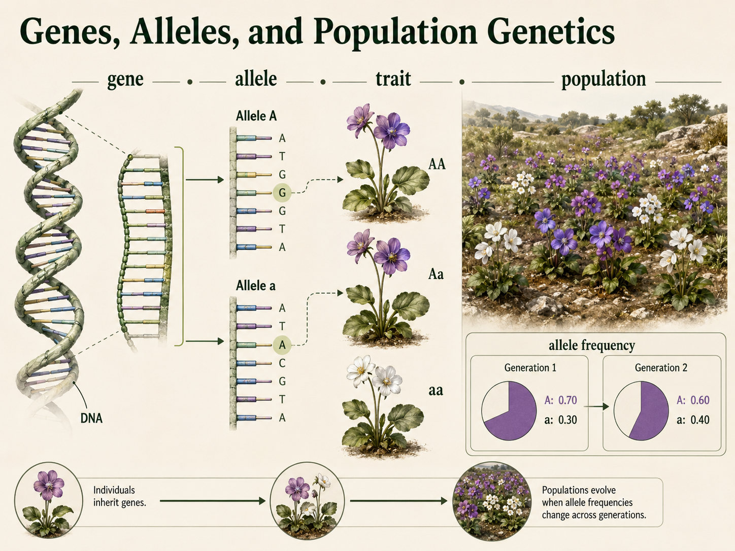
Figure 1. Genes, Alleles, and Population Genetics. A gene is a segment of DNA that influences a trait, and alleles are different versions of the same gene. Population genetics studies how common different alleles are in a population and how allele frequencies change across generations.
The Gene Pool Concept
The gene pool is the complete collection of alleles present in a population. It includes all copies of all alleles carried by all individuals in that population. In sexually reproducing diploid organisms, most individuals carry two copies of each autosomal gene, one inherited from each parent. A gene pool can be imagined as all the genetic variation available to be passed into the next generation. The Hardy-Weinberg model focuses on a simplified case: one gene with two alleles in a sexually reproducing population. This model is simple, but powerful, because it shows how allele frequencies are related to genotype frequencies. Real populations are often more complicated. Many traits are influenced by multiple genes, populations may be divided into subgroups, and several evolutionary forces may act at the same time. Even so, the gene pool concept is essential because it shifts the focus from individual inheritance to genetic change across an entire population.
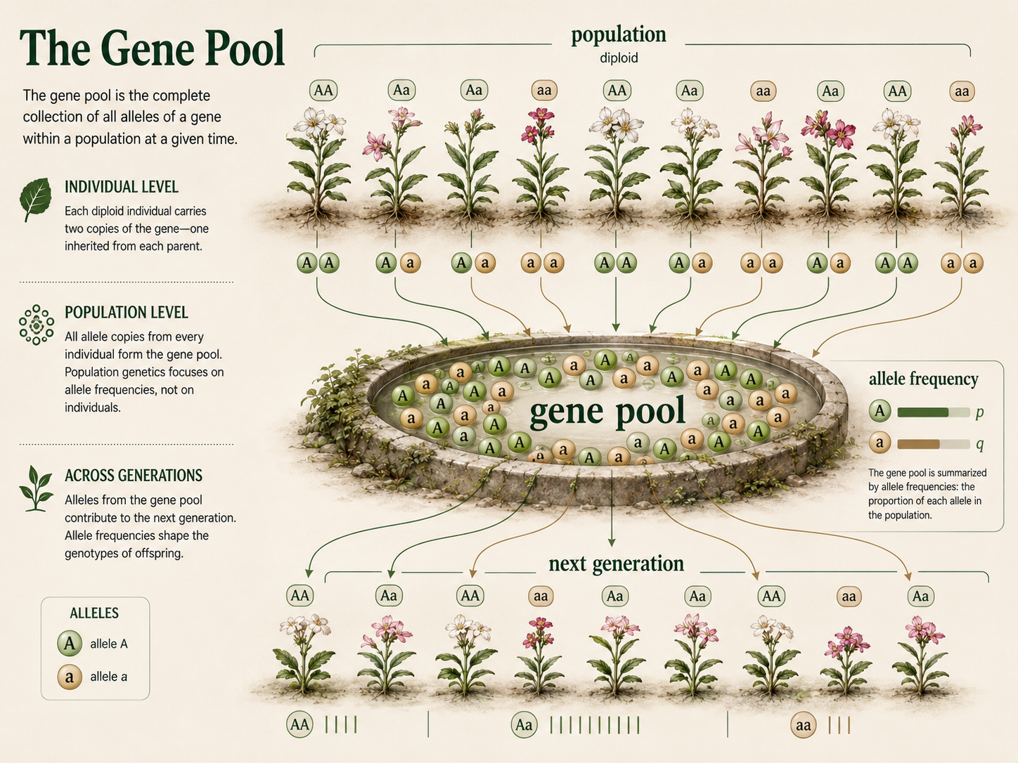
Figure 2. The Gene Pool. The gene pool is the complete collection of alleles present in a population. In diploid organisms, individuals usually carry two copies of each autosomal gene, and population genetics studies how the frequencies of those alleles change across generations.
Allele Frequencies and Genotype Frequencies
An allele frequency is the proportion of all gene copies in a population represented by a particular allele. For example, if 70 out of 100 copies of a gene are allele A, then the frequency of allele A is 0.70, or 70%. Allele frequencies are calculated by counting alleles, not individuals. In a simple two-allele model, the frequency of one allele is represented by p (e.g. %A), and the frequency of the other allele is represented by q (e.g. %a). Since these are the only two alleles in the model, their frequencies must add up to 1. Mathematically: p + q =1. For example, if the frequency of allele A is 0.70, then p = 0.7, the frequency of allele a must be 0.30, so q = 0.3. A homozygous individual (e.g. AA and aa) contributes two copies of the same allele to the gene pool, while a heterozygous individual (e.g. Aa) contributes one copy of each allele. A genotype frequency is the proportion of individuals in a population with a particular genotype. Genotype frequencies are calculated by counting individuals with each genotype. For example, if 42 out of 100 individuals have the genotype Aa, then the frequency of the Aa genotype is 0.42, or 42%. Allele frequencies and genotype frequencies are related, but they are not the same. Allele frequencies describe how common each allele is in the gene pool, while genotype frequencies describe how common each genotype is among individuals in the population.

Figure 3. Allele Frequencies and Genotype Frequencies. Allele frequency describes how common an allele is among all gene copies in a population, while genotype frequency describes how common a genotype is among individuals. These measures are related, but they are calculated differently and describe different levels of genetic variation.
The Hardy-Weinberg Principle
The Hardy-Weinberg principle predicts genotype frequencies from allele frequencies when a population is not evolving at a particular gene. Mendel focused on how alleles are passed from parents to offspring. Hardy and Weinberg extended this idea to the population level by asking a larger question: what should happen to allele frequencies from one generation to the next if evolution is not occurring? For a gene with two alleles, p represents the frequency of one allele (e.g. %A) and q represents the frequency of the other allele (e.g. %a). The Hardy-Weinberg principle predicts allele frequencies will not change from one generation to the next if 1) mating is random and 2) no evolutionary forces are acting.
Hardy-Weinberg as a Null Model
The Hardy-Weinberg principle is best understood as a null model. A null model describes what we would expect if no major process were changing the system. In this case, Hardy-Weinberg equilibrium describes what genotype frequencies should look like if mating is random in a population and it is not evolving at the gene being studied. In the case of this null model, if the genotype frequencies do not match what the Hardy-Weinberg model predicts it indicates that one or both of these assumptions have not been met. In other words, either mating is not random or natural selection is occurring, or both. This does not mean real populations usually meet all Hardy-Weinberg assumptions perfectly. They often do not. That is exactly why the model is useful. Scientists can compare observed genotype frequencies in a real population to expected Hardy-Weinberg frequencies. If the observed and expected values are very different, that difference suggests that something is happening in the population. The cause might be natural selection, genetic drift, gene flow, mutation, nonrandom mating, or hidden population structure. Hardy-Weinberg equilibrium is not just a math equation. It is a baseline that helps scientists detect evolutionary change.
Assumptions of the Hardy-Weinberg Model
For a population to remain in Hardy-Weinberg equilibrium, two assumptions must be met. First, mating must be random with respect to the gene being studied, meaning individuals do not choose mates based on traits related to that gene. Second, there must be no natural selection, meaning all genotypes survive and reproduce equally well. If any of these assumptions are violated, allele frequencies may change over time. That change is evolution. These assumptions are not meant to describe a perfect real-world population. They are meant to help us identify the forces that cause populations to evolve.
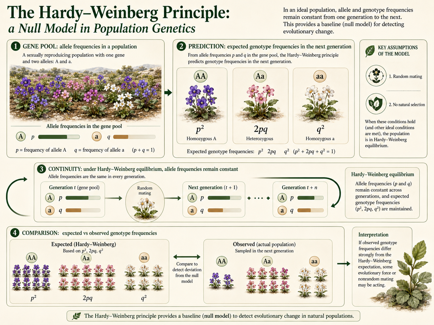
Figure 4. The Hardy-Weinberg Principle. The Hardy-Weinberg principle predicts genotype frequencies from allele frequencies when a population is not evolving at a particular gene. It serves as a null model: if observed genotype frequencies differ from Hardy-Weinberg expectations, then random mating, equal survival and reproduction, or both may not be occurring, suggesting evolutionary change.
Predicting Genotype Frequencies with the Hardy-Weinberg Equation
If mating is random and no evolutionary forces are acting on the population, allele frequencies remain constant from generation to generation, and genotype frequencies can be predicted from those allele frequencies. The equation p² + 2pq + q² = 1 predicts the expected genotype frequencies in a population under Hardy-Weinberg equilibrium. Assuming only two possible alleles for each gene, then p + q = 1, where p represents the frequency of one allele (e.g. A), and q represents the frequency of the other allele (e.g. a). This equation is based on the probability of alleles combining during fertilization. If the frequency of allele A (%A) is p, then the probability (assuming random mating) of an offspring receiving an A allele from both parents is p × p, or p². This represents the expected frequency of homozygous dominant individuals (p² = %AA). If the frequency of allele a is q, then the probability of receiving an a allele from both parents is q × q, or q². This represents the expected frequency of homozygous recessive individuals (q² = %aa). A heterozygous individual, Aa, can form in two ways: an A allele from one parent and an a allele from the other, or an a allele from one parent and an A allele from the other. Because there are two possible ways to make a heterozygote, the expected frequency of heterozygous individuals is (2pq = %Aa). Together, these values add up to 1, or 100% of the population, giving us p² + 2pq + q² = 1. The Hardy-Weinberg model therefore makes two important predictions: genotype frequencies can be predicted from allele frequencies, and allele frequencies will remain constant across generations if the assumptions of the model are met. If it is found that a population’s allele frequency does not remain constant, then it is assumed that one or both of the assumptions have not been met. In other words, either 1) mating was not random or 2) natural selection has occurred, or 3) both occurred (mating was not random and natural selection has also occurred).

Figure 5. Predicting Genotype Frequencies with the Hardy-Weinberg Equation. Under Hardy-Weinberg equilibrium, allele frequencies can be used to predict expected genotype frequencies. If p is the frequency of allele A and q is the frequency of allele a, then p² predicts AA, 2pq predicts Aa, and q² predicts aa. Together, these genotype frequencies add up to 1, or 100% of the population.
Example Calculation from Allele Frequencies
Imagine a population in which the frequency of allele A is 0.7 and the frequency of allele a is 0.3. In Hardy-Weinberg terms, p = 0.7 and q = 0.3. The expected frequency of the AA genotype is p². The expected frequency of the Aa genotype is 2pq. The expected frequency of the aa genotype is q². These genotype frequencies add up to 1.00, or 100% of the population. This means that 49% of the population is expected to be AA (p² = 0.49) , 42% is expected to be Aa (2pq = 0.42), and 9% is expected to be aa (q² = 0.09). If the population is in Hardy-Weinberg equilibrium, the allele frequencies in the next generation will remain 0.7 for allele A and 0.3 for allele a. Sexual reproduction reshuffles alleles into new genotype combinations, but reshuffling alone does not change allele frequencies.
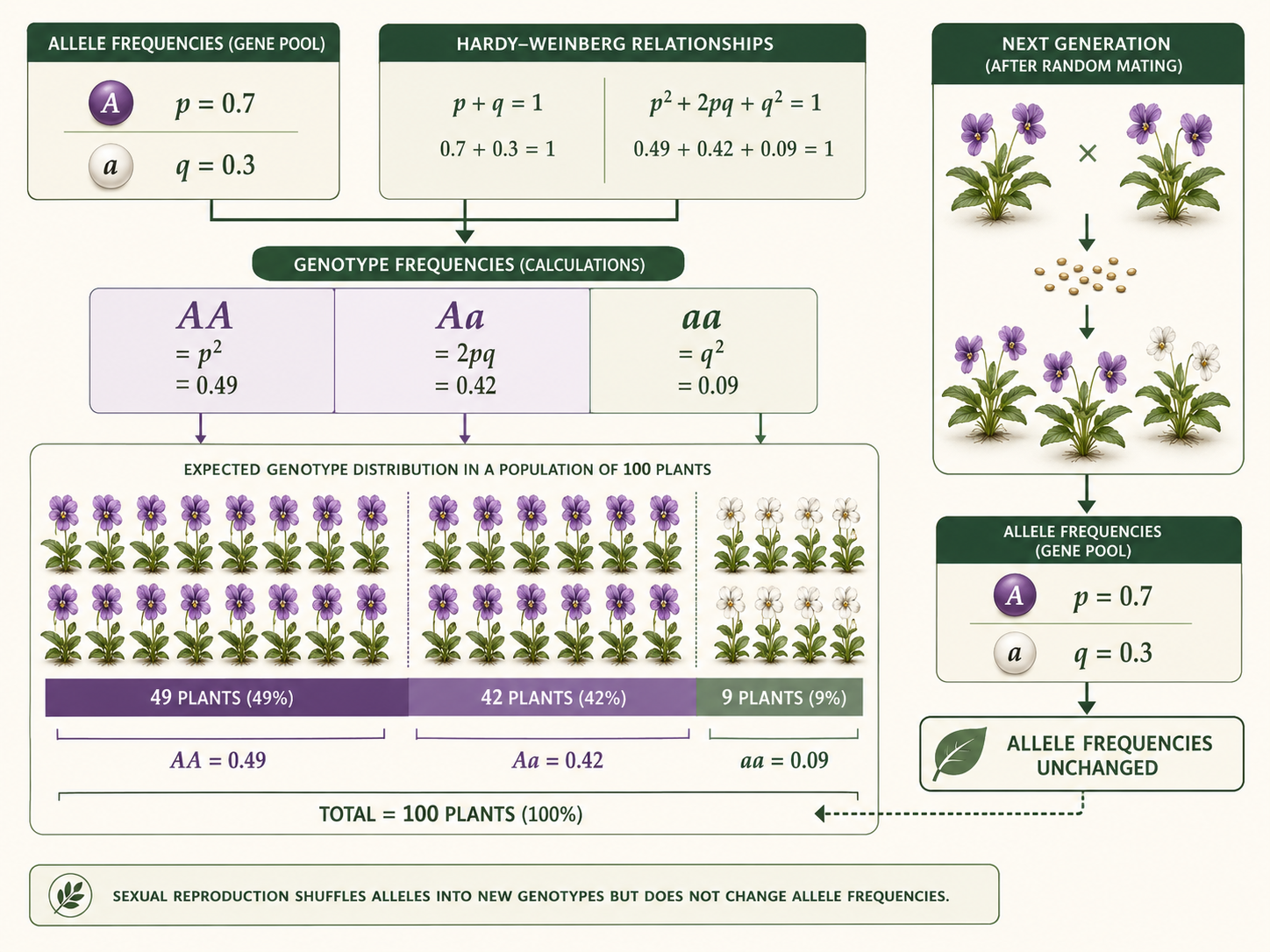
Figure 6. Example Calculation from Allele Frequencies. If p = 0.7 and q = 0.3, the Hardy-Weinberg equation predicts genotype frequencies of 0.49 for AA, 0.42 for Aa, and 0.09 for aa. These values add to 1.00, or 100% of the population.
Practice Predicting Hardy-Weinberg Frequencies
In the activity below, you will practice using the Hardy-Weinberg equations to predict allele, genotype, and phenotype frequencies. A random value for p, the frequency of the dominant allele A, has been generated for you. Your job is to use that value to calculate q, the frequency of the recessive allele a, and then predict the expected frequencies of AA, Aa, and aa genotypes. After entering your predictions, submit your answers to check your work. The activity will show which answers are correct, explain any mistakes, and display the full calculation steps. Remember that the dominant phenotype includes both AA and Aa individuals, while the recessive phenotype includes only aa individuals.
Testing Hardy-Weinberg Equilibrium in the Real World with Chi-Square Analysis
Scientists can test whether a population is in Hardy-Weinberg equilibrium by comparing the observed genotype frequencies (those actually measured) in a population with the genotype frequencies expected under the Hardy-Weinberg model. The basic question is: do the data from this population match what we would expect if allele frequencies are stable and no evolutionary forces are acting on this gene? To begin, scientists collect data from a population and count how many individuals have each genotype. For a gene with two alleles, A and a, the observed genotype counts might be AA, Aa, and aa. These observed genotype counts can then be used to calculate the observed allele frequencies. The frequency of the dominant allele A is called p, and the frequency of the recessive allele a is called q. Because each individual has two alleles for the gene, allele frequencies are calculated from the total number of allele copies in the population, not just from the number of individuals. For example, imagine a population of 200 individuals with the following observed genotype counts:
Because there are 200 individuals, there are 400 total allele copies. Each AA individual has two A alleles, each Aa individual has one A allele and one a allele, and each aa individual has two a alleles. The allele frequencies are calculated like this:
Once scientists know p and q, they use the Hardy-Weinberg equation to calculate the expected genotype frequencies:
These are expected frequencies, but a chi-square test compares observed and expected counts, not just frequencies. To convert the expected frequencies into expected counts, multiply each expected frequency by the total population size, which is 200:
At this point, scientists use a chi-square test to determine whether the differences between the observed and expected counts are small enough to be explained by chance, or large enough to suggest that the population may not be in Hardy-Weinberg equilibrium. The chi-square formula is:
For this example:
The total chi-square value is:
The chi-square value is then compared with a critical value from a chi-square table. For a Hardy-Weinberg test with two alleles and three genotype categories, the degrees of freedom are usually 1 because the allele frequencies are estimated from the observed data. At the 0.05 significance level, the critical value for 1 degree of freedom is 3.84. In this example, the chi-square value is 2.92. Because 2.92 is less than 3.84, the difference between the observed and expected genotype counts is not large enough to reject Hardy-Weinberg equilibrium. This means the population does not show strong evidence that allele frequencies are changing at this gene. The key idea is simple: a small chi-square value means the observed data are close to the expected values. A large chi-square value means the observed data are very different from the expected values. If the difference is large enough, scientists reject Hardy-Weinberg equilibrium and look for possible causes, such as natural selection, genetic drift, gene flow, mutation, nonrandom mating, or population structure.
The figure below is a summary of this example.
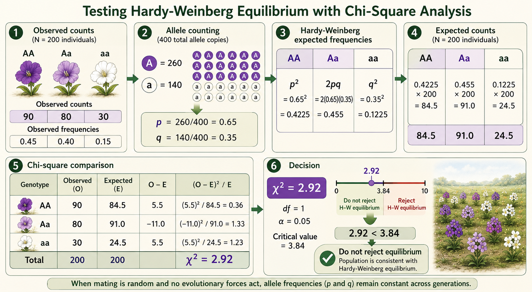
Figure 7. Testing Hardy-Weinberg Equilibrium with Chi-Square Analysis. Scientists test Hardy-Weinberg equilibrium by comparing observed genotype counts with expected genotype counts predicted from allele frequencies. In this example, χ² = 2.92 is less than the critical value of 3.84, so the observed differences are not large enough to reject Hardy-Weinberg equilibrium.
Practice Testing Hardy-Weinberg Equilibrium with Chi-Square Analysis
In this activity, you will practice using a chi-square test to evaluate whether a population fits Hardy-Weinberg expectations. You can adjust the population size and the target allele frequency for p, then generate a sample of observed genotype counts. The activity will calculate the observed allele frequencies, the expected genotype frequencies, the expected genotype counts, and the final chi-square value. Your job is to interpret the result. Compare the chi-square value to the critical value of 3.84. If the chi-square value is less than or equal to 3.84, the observed data are close enough to the expected data that Hardy-Weinberg equilibrium is not rejected. If the chi-square value is greater than 3.84, the observed and expected genotype counts are different enough to reject Hardy-Weinberg equilibrium. In that case, the population may be affected by nonrandom mating, natural selection, or another evolutionary force.
Using Phenotype Data Carefully in Hardy-Weinberg Analysis
Phenotype measurements can also be useful, but they must be interpreted carefully. If A is completely dominant over a, then individuals with AA and Aa genotypes have the same dominant phenotype. Only individuals with the aa genotype show the recessive phenotype. This means phenotype counts can identify the recessive genotype directly, but they cannot separate homozygous dominant individuals from heterozygotes. For example, if 170 individuals show the dominant phenotype and 30 show the recessive phenotype, scientists know that the 30 recessive individuals are likely aa, but the 170 dominant individuals include both AA and Aa. Because of this, direct genotype data are usually better for a Hardy-Weinberg chi-square test. Phenotype data can still be used to estimate allele frequencies, especially when the recessive phenotype represents q², but the conclusions are less direct.

Figure 8. Using Phenotype Data Carefully in Hardy-Weinberg Analysis. Phenotype data can identify the recessive genotype when the recessive phenotype represents aa, but dominant phenotypes may include both AA and Aa individuals. Because phenotype counts cannot always separate genotypes, direct genotype data are usually better for Hardy-Weinberg chi-square tests.
Evolutionary Forces
An evolutionary force is any process that changes allele frequencies in a population over time. The major evolutionary forces are natural selection, genetic drift, gene flow, and mutation. Natural selection changes allele frequencies when individuals with certain heritable traits survive or reproduce more successfully than others. Genetic drift changes allele frequencies by random chance, especially in small populations. Gene flow changes allele frequencies when alleles move between populations. Mutation creates new alleles by changing DNA sequences. Nonrandom mating can change genotype frequencies, and sexual selection can strongly affect which alleles are passed to future generations. These forces can act separately or together. For example, a small island population may experience genetic drift because it is small, natural selection because some traits improve survival, mutation because new alleles occasionally arise, and gene flow if individuals arrive from another island. Population genetics studies how these forces shape genetic variation.
Natural Selection
Natural selection occurs when individuals with certain heritable traits survive or reproduce more successfully than others. If those traits are genetically influenced, the alleles associated with them may become more common in future generations. Natural selection is not random, but it also does not have a goal. It favors traits that increase fitness in a particular environment. A trait that is beneficial in one environment may be harmful or neutral in another. For example, alleles that improve heat tolerance may be useful in a hot climate but provide little advantage in a cool climate. Antibiotic resistance in bacteria is another clear example. When antibiotics are used, bacteria with resistance alleles are more likely to survive and reproduce. Over time, resistance alleles become more common in the bacterial population. Natural selection acts on phenotypes, but evolution occurs when the genetic basis of those phenotypes changes in frequency. Selection affects individuals, but populations evolve.
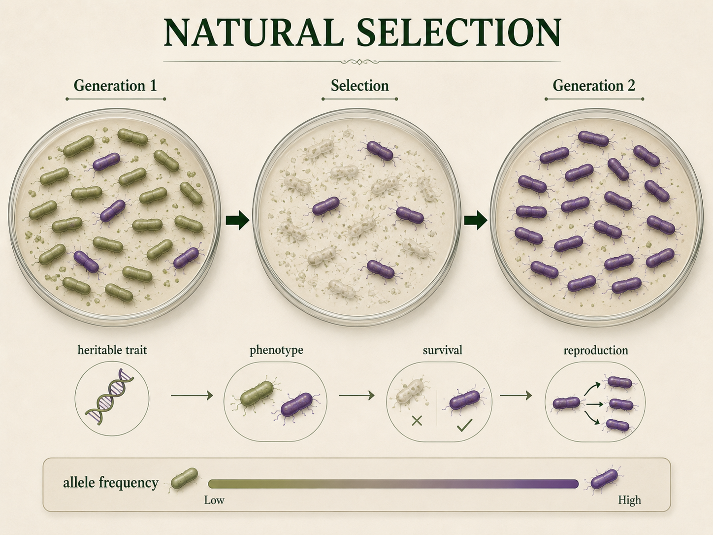
Figure 8. Natural Selection. Natural selection occurs when individuals with certain heritable traits survive or reproduce more successfully than others. Selection acts on phenotypes, but populations evolve when the alleles associated with those phenotypes change in frequency.
Types of Natural Selection
Natural selection can affect trait variation in several major ways. Directional selection favors one extreme phenotype, causing the average trait value in a population to shift in one direction. Antibiotic resistance in bacteria and pesticide resistance in insects are strong examples because resistant individuals survive chemical exposure and pass resistance alleles to future generations. Stabilizing selection favors intermediate phenotypes and selects against extreme phenotypes, reducing variation around the average. Human birth weight is often used as an example because very low and very high birth weights can both be associated with increased risk, although modern medicine can alter these patterns. Disruptive selection favors individuals at both extremes of a trait and selects against intermediate phenotypes. This can increase variation within a population and, under some conditions, contribute to speciation. A useful example involves seed-eating birds in environments where small and large seeds are common, but medium-sized seeds are rare. Birds with small or large beaks may feed efficiently, while birds with intermediate beaks may be less effective.
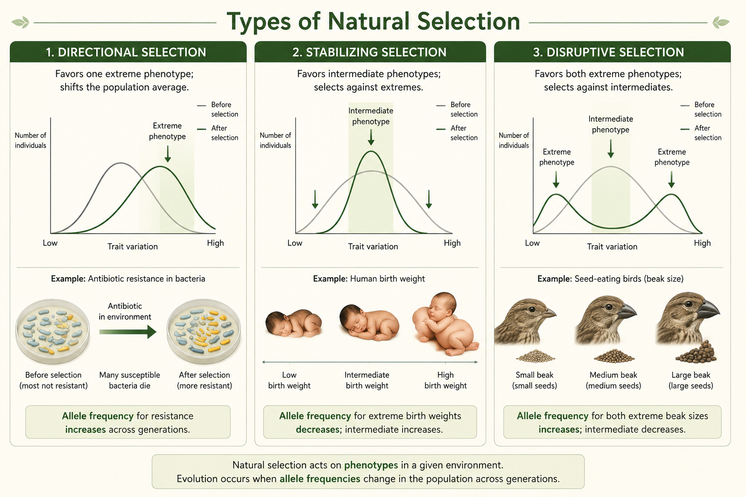
Figure 9. Types of Natural Selection. Directional selection favors one extreme phenotype, stabilizing selection favors intermediate phenotypes, and disruptive selection favors both extremes. These patterns change trait variation depending on which phenotypes have the highest fitness in a particular environment.
Balancing Selection
Balancing selection occurs when natural selection maintains more than one allele in a population. This is important because selection does not always remove variation. Sometimes selection preserves genetic diversity. One form of balancing selection is heterozygote advantage, where heterozygous individuals have higher fitness than either homozygous genotype. The classic example is the sickle-cell allele in regions where malaria is common. Individuals with two normal hemoglobin alleles are more vulnerable to malaria. Individuals with two sickle-cell alleles can develop sickle-cell disease. Heterozygous individuals have some protection against malaria without usually having the most severe form of sickle-cell disease. As a result, both alleles can remain in the population. Another form of balancing selection is frequency-dependent selection, where the fitness of a phenotype depends on how common or rare it is. In some cases, rare phenotypes have an advantage because predators, parasites, or competitors are less adapted to them.
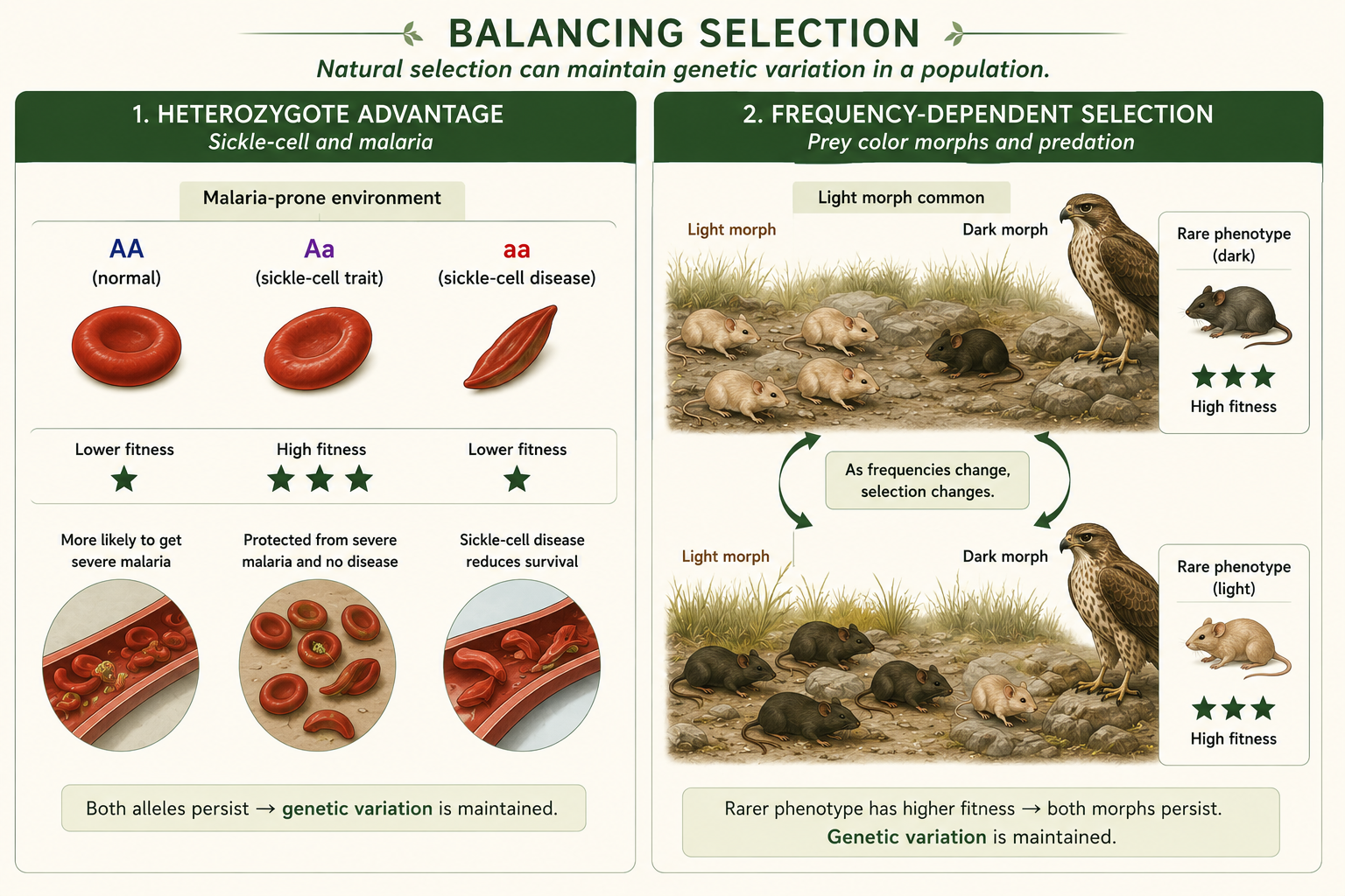
Figure 10. Balancing Selection. Balancing selection maintains more than one allele in a population. It can occur through heterozygote advantage or through frequency-dependent selection, where rare phenotypes may have higher fitness.
Genetic Drift
Genetic drift is random change in allele frequencies from one generation to the next. Unlike natural selection, genetic drift does not favor alleles because they are helpful. It occurs because reproduction is partly a matter of chance. By random luck, some individuals leave more offspring than others. When that happens, some alleles become more common and others become less common. Genetic drift is strongest in small populations because chance events have a larger effect when there are fewer individuals. Over time, genetic drift can cause alleles to become fixed or lost. An allele becomes fixed when it is the only allele left at that gene in the population. An allele is lost when it disappears from the population. Genetic drift usually reduces genetic variation within populations. It can also make different populations more genetically different from one another. This is especially important in endangered species, island populations, and isolated habitat fragments.
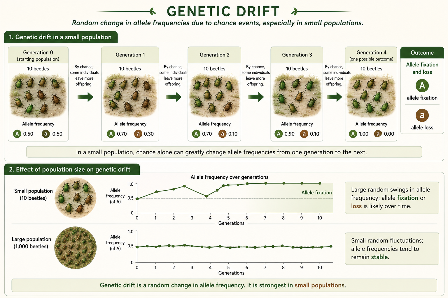
Figure 11. Genetic Drift. Genetic drift is random change in allele frequencies from one generation to the next. It is strongest in small populations and can cause alleles to become fixed or lost, often reducing genetic variation within populations.
Founder Effect and Population Bottlenecks
Two important examples of genetic drift are the founder effect and the population bottleneck. The founder effect occurs when a small number of individuals establish a new population. Because the founders carry only a small sample of the original population’s genetic variation, the new population may have allele frequencies that differ greatly from the source population. This can happen when organisms colonize islands, isolated lakes, or newly available habitats. A population bottleneck occurs when a population is suddenly reduced to a very small size. This may happen because of disease, natural disaster, overhunting, habitat destruction, or climate stress. Even if the population later grows again, much of its original genetic variation may be lost. Bottlenecks can increase inbreeding and reduce the ability of a population to adapt to future environmental change. Both founder effects and bottlenecks show that populations can evolve by chance, not only by natural selection.
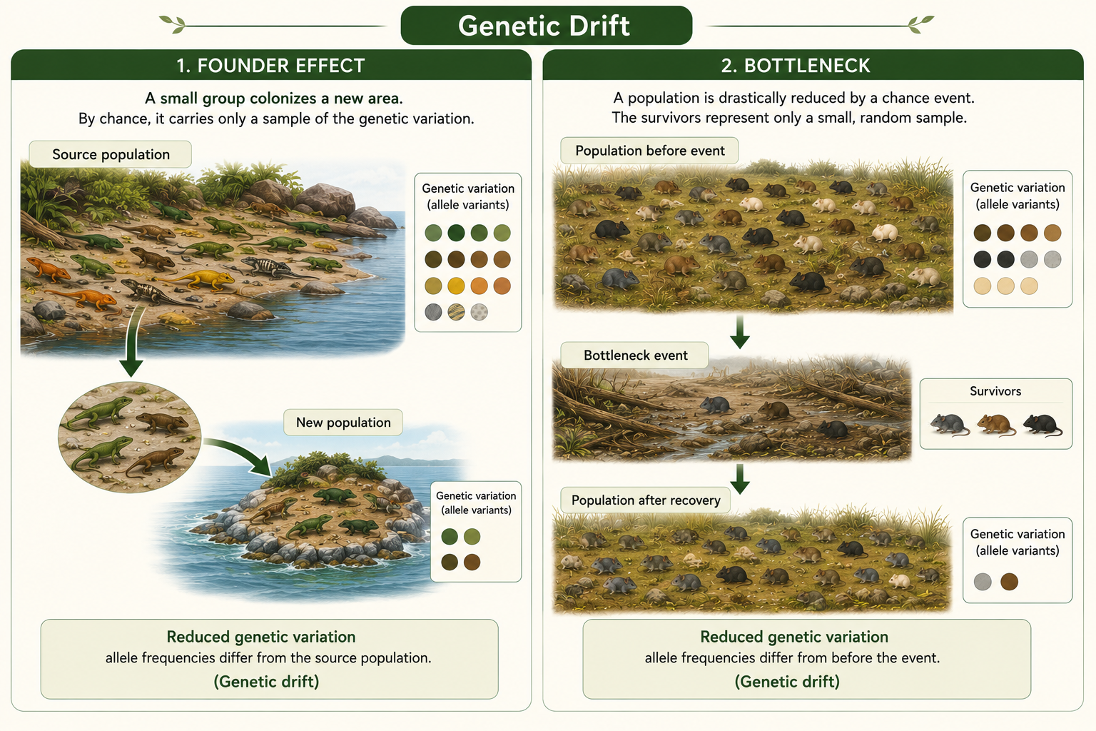
Figure 12. Founder Effect and Population Bottlenecks. The founder effect occurs when a small group starts a new population with only part of the original genetic variation. A bottleneck occurs when a population is sharply reduced, often leaving fewer alleles in later generations.
Gene Flow
Gene flow is the movement of alleles between populations. It occurs when individuals migrate from one population to another and successfully reproduce. It can also occur when gametes move between populations, such as pollen moving between plant populations. Gene flow can introduce new alleles into a population and increase genetic variation. It can also make different populations more genetically similar to one another. In this way, gene flow can slow or oppose speciation because it reduces genetic differences between populations. For example, if two populations of the same species live in different habitats but individuals frequently move and reproduce between them, the populations may remain genetically similar. However, if gene flow is reduced or stopped, genetic drift, mutation, and natural selection can cause the populations to diverge over time. Gene flow is therefore important for both maintaining genetic diversity and understanding how populations become reproductively isolated.
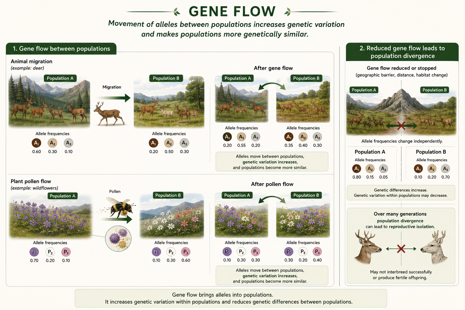
Figure 13. Gene Flow. Gene flow is the movement of alleles between populations through migration, reproduction, or gamete movement such as pollen dispersal. It can introduce new alleles, increase genetic variation, and make populations more genetically similar.
Mutations
A mutation is a change in DNA sequence. Mutations are the original source of new alleles. Without mutation, there would be no new genetic variation for natural selection, genetic drift, or other evolutionary forces to act on. Many mutations are neutral, meaning they have little or no effect on fitness. Some mutations are harmful, especially if they disrupt important genes. A smaller number may be beneficial in a particular environment. Mutation is especially important over long timescales because it continually introduces new variation into populations. In asexual organisms such as bacteria, mutation is a major source of new genetic differences among lineages. In sexually reproducing organisms, mutation creates new alleles, while meiosis and recombination shuffle existing alleles into new combinations. Mutation alone usually changes allele frequencies slowly, but it is essential because it provides the raw material for evolution.
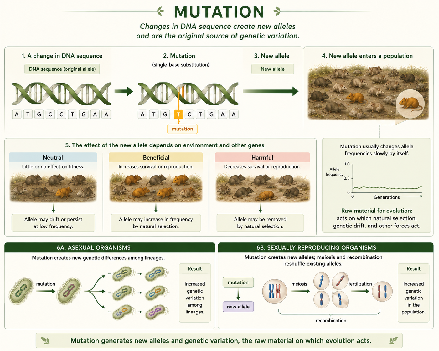
Figure 14. Mutations. Mutation is a change in DNA sequence and the original source of new alleles. Although many mutations are neutral and mutation alone often changes allele frequencies slowly, it provides the genetic variation that other evolutionary forces act on.
Recombination and Genetic Variation
Recombination occurs during meiosis when chromosomes exchange segments of DNA. Recombination does not usually create brand-new alleles, but it does create new combinations of alleles. This matters because natural selection often acts on combinations of traits, not isolated genes. Sexual reproduction also increases genetic variation through independent assortment and fertilization. Independent assortment randomly distributes maternal and paternal chromosomes into gametes. Fertilization combines alleles from two parents. Together, mutation, recombination, independent assortment, and fertilization generate genetic variation among offspring. This variation matters because populations with more genetic diversity usually have greater potential to respond to changing environments. A population with very little genetic variation may survive under current conditions but struggle if climate, disease, predators, or resources change.
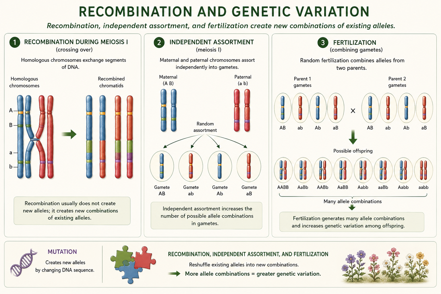
Figure 15. Recombination and Genetic Variation. Recombination occurs during meiosis when chromosomes exchange DNA segments, creating new combinations of alleles. Independent assortment and fertilization further increase genetic variation among offspring.
Nonrandom Mating and Inbreeding
Nonrandom mating occurs when individuals do not pair by chance. Individuals may choose mates based on size, color, song, territory quality, relatedness, timing, or location. Nonrandom mating does not necessarily change allele frequencies by itself, but it can change genotype frequencies. One important form of nonrandom mating is inbreeding, which occurs when closely related individuals mate. Inbreeding increases homozygosity, meaning individuals are more likely to inherit two copies of the same allele from a common ancestor. This can expose harmful recessive alleles and reduce fitness, a pattern called inbreeding depression. Inbreeding is a serious concern in small, isolated, or endangered populations. Conservation biologists often try to maintain gene flow among populations to reduce inbreeding and preserve genetic diversity. This is another reason population genetics is important for protecting threatened species.
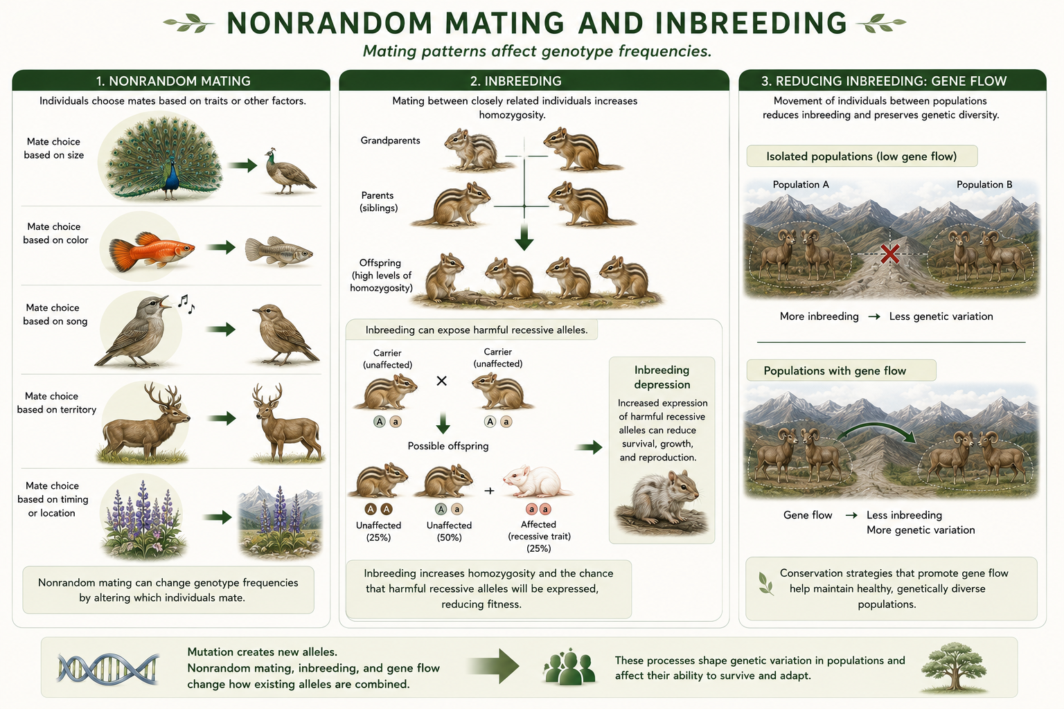
Figure 16. Nonrandom Mating and Inbreeding. Nonrandom mating occurs when individuals do not pair by chance and can change genotype frequencies. Inbreeding increases homozygosity, which can expose harmful recessive alleles and reduce fitness in small or isolated populations.
Sexual Selection and Dimorphism
Sexual selection is a form of natural selection that occurs when individuals differ in their ability to obtain mates. Some traits increase mating success even if they are costly for survival. For example, bright coloration, elaborate songs, large antlers, or complex courtship displays can make individuals more attractive to mates or more successful in competition. However, these traits may also require energy or increase the risk of predation. Sexual selection often occurs through mate choice, where one sex chooses among potential mates, and intrasexual competition, where individuals of the same sex compete for access to mates. Sexual selection can lead to sexual dimorphism, which means males and females of the same species differ in size, color, shape, or behavior. In many bird species, males are more brightly colored than females, but patterns vary widely depending on ecology, parental investment, and mating system. The key point is that sexual selection can change allele frequencies by affecting reproductive success.
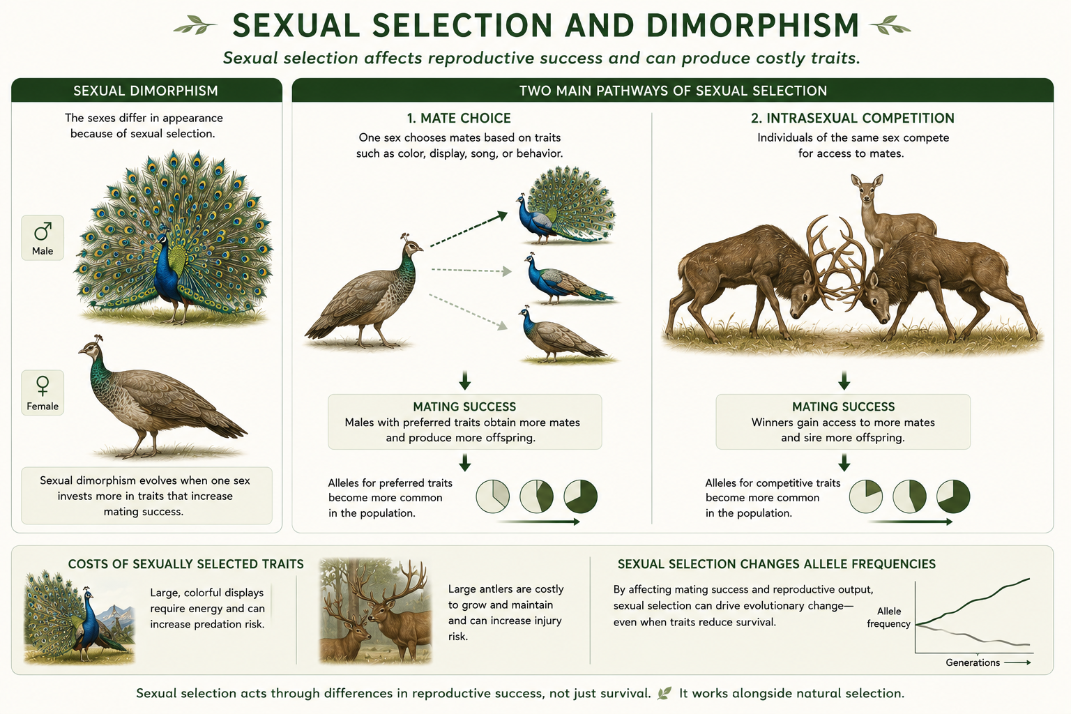
Figure 17. Sexual Selection and Dimorphism. Sexual selection occurs when individuals differ in their ability to obtain mates. Traits such as bright coloration, elaborate displays, songs, or antlers can increase mating success even if they carry survival costs.
Population Genetics and Speciation
Population genetics helps explain how new species form. Speciation often begins when populations of the same species become genetically different over time. This can happen when populations are geographically separated, experience different selective pressures, undergo genetic drift, or lose gene flow between them. Gene flow tends to keep populations similar, while mutation, natural selection, and genetic drift can make them different. If populations remain separated long enough, they may accumulate genetic differences that affect mating behavior, fertility, development, timing of reproduction, or survival of hybrid offspring. Eventually, the populations may become reproductively isolated, meaning they no longer successfully interbreed. At that point, they may be considered separate species. This shows the connection between microevolution and macroevolution. Small changes in allele frequencies within populations can accumulate over time and contribute to the origin of new species. We will expand on the concept of speciation in the next chapter.
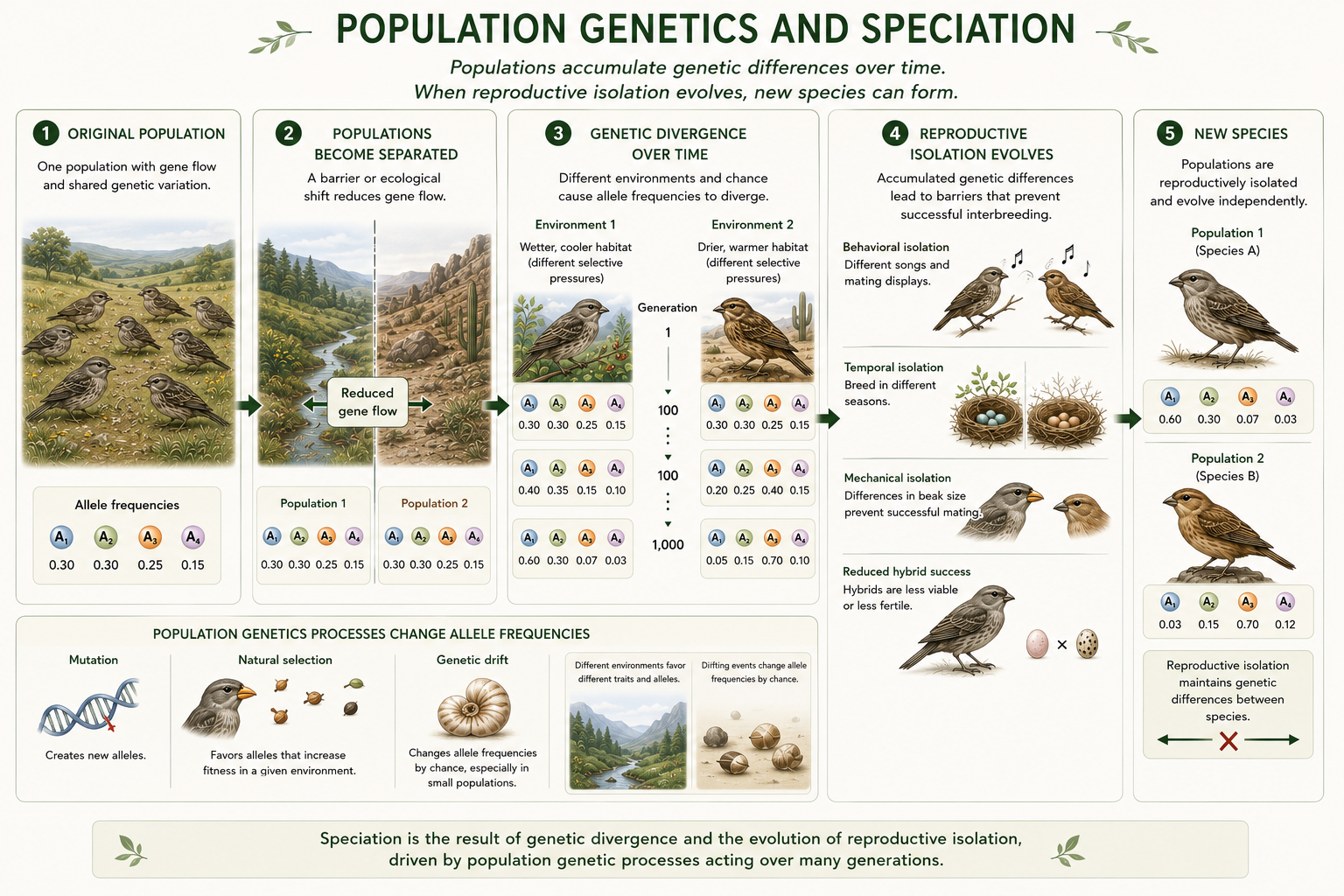
Figure 18. Population Genetics and Speciation. Speciation can begin when populations lose gene flow and accumulate genetic differences through mutation, natural selection, and genetic drift. Over time, these differences may lead to reproductive isolation and the formation of separate species.