
Chapter: Population Ecology
Population ecology is the study of how and why populations change over time. In ecology, a population is a group of individuals of the same species living in the same area at the same time. A population might be all the white-tailed deer in a forest, all the oak trees in a park, all the bacteria in a pond, or all the humans living in a city. Population ecologists study patterns of birth, death, immigration, emigration, survival, reproduction, density, age structure, and growth. They often use mathematics because populations change in measurable ways. Mathematical models do not capture every detail of nature, but they help ecologists make predictions, compare populations, and understand the forces that cause populations to increase, decrease, or remain stable. Population ecology is important because it helps scientists understand endangered species, invasive species, disease spread, wildlife management, fisheries, agriculture, conservation, and human population growth. At its core, population ecology asks a simple but powerful question: what causes the number of individuals in a population to change?
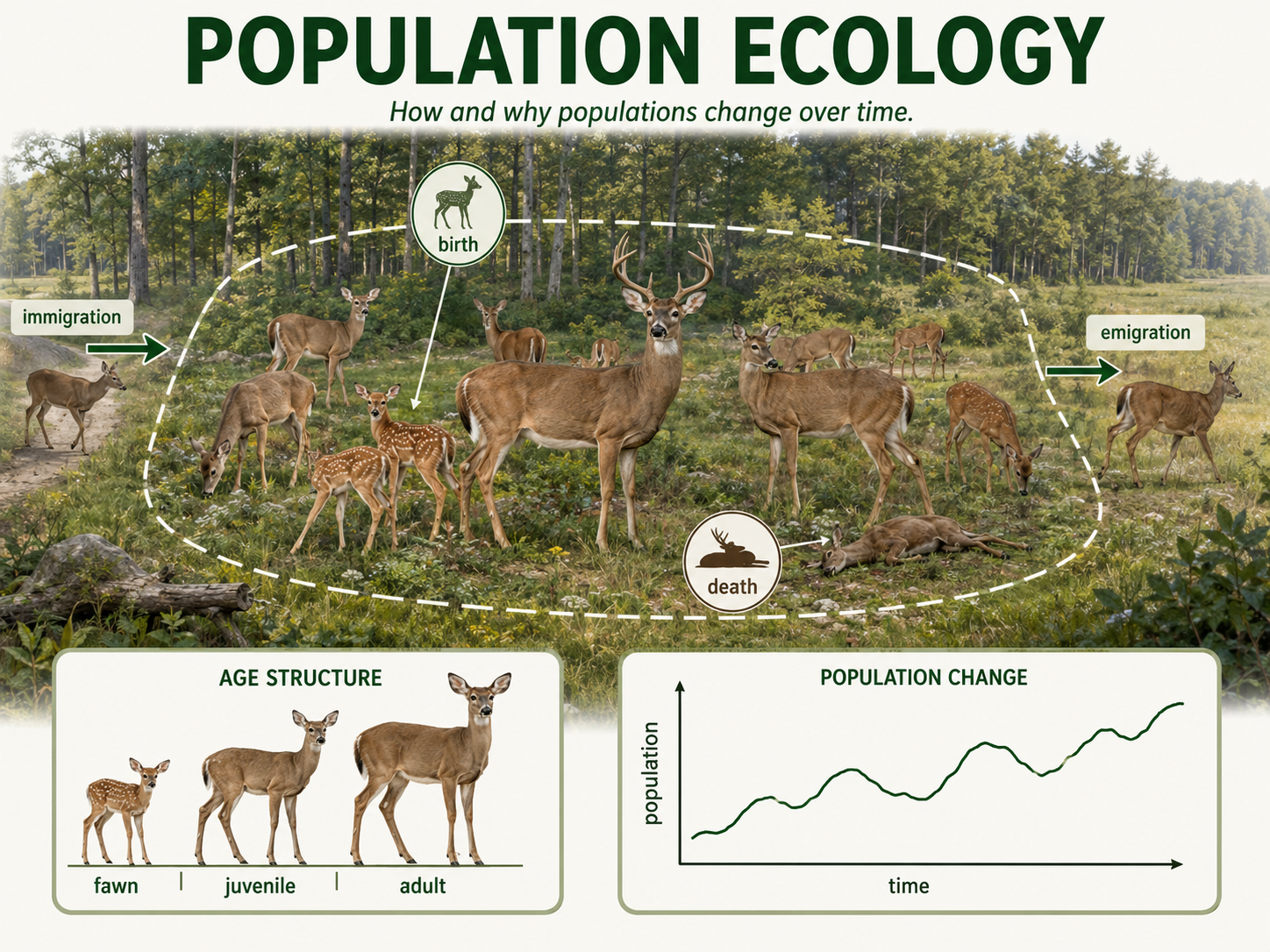
Figure 1. Population Ecology. Population ecology is the study of how and why populations change over time. Ecologists study births, deaths, immigration, emigration, survival, reproduction, density, age structure, and growth to understand whether populations increase, decrease, or remain stable.
Demography
Demography is the study of the size, structure, and changes of populations through time. A population increases when individuals are added through births and immigration, and it decreases when individuals are removed through deaths and emigration. Immigration means individuals move into a population. Emigration means individuals move out of a population. A simple way to describe population change is: new population size equals old population size plus births, minus deaths, plus immigration, minus emigration. This can be written as: N₂ = N₁ + B − D + I − E, where N₁ is the starting population size, N₂ is the later population size, B is births, D is deaths, I is immigration, and E is emigration. If births and immigration are greater than deaths and emigration, the population grows. If deaths and emigration are greater than births and immigration, the population declines. Demography gives ecologists the basic accounting system for understanding population change. It also reminds us that population growth is not only about reproduction. Movement matters too. A population can grow even if births are low, as long as enough individuals immigrate into the area. A population can also decline even if reproduction occurs, especially if death rates are high or many individuals leave.
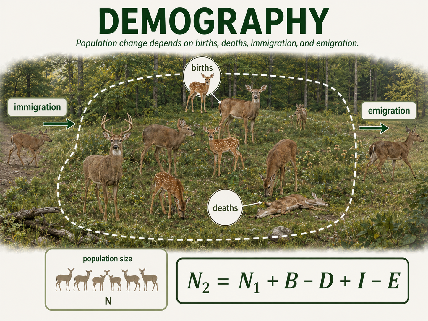
Figure 2. Demography. Demography tracks how population size changes through births, deaths, immigration, and emigration. A population grows when additions exceed losses and declines when losses exceed additions.
Population Size and Population Density
Population size is the total number of individuals in a population. Population density is the number of individuals per unit area or volume. For example, a forest might contain 500 pine trees total, but ecologists may also want to know whether those trees are spread over one hectare or ten hectares. Density matters because many ecological processes depend on how crowded a population is. High density can increase competition, disease transmission, and stress, but it can also make it easier to find mates or defend against predators. Low density can reduce competition, but it can make reproduction more difficult if individuals have trouble finding mates. This is one reason population ecology often focuses not just on how many individuals exist, but also on how closely they are packed together. Density can also affect behavior. Crowded animals may defend territories more aggressively, plants may grow taller as they compete for light, and disease may spread more quickly when individuals are close together. Population size tells us how many organisms are present; population density helps explain how strongly those organisms interact.
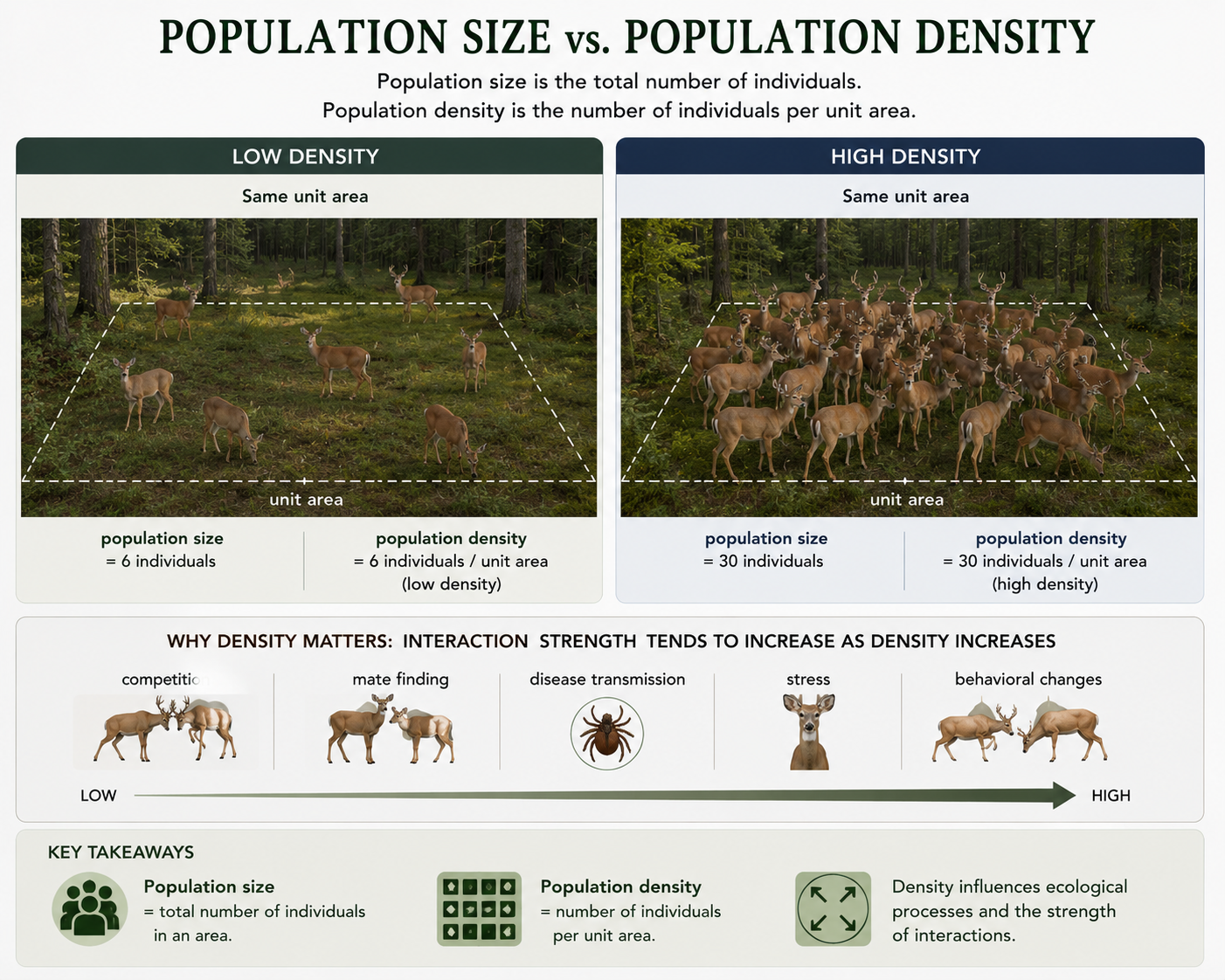
Figure 3. Population Size and Population Density. Population size is the total number of individuals in a population, while population density is the number of individuals per unit area or volume. Density affects how strongly individuals interact through competition, reproduction, disease transmission, and behavior.
Estimating Population Size
Ecologists often cannot count every individual in a population, especially when organisms are small, mobile, hidden, or spread across a large area. Instead, they estimate population size using sampling methods. For plants or slow-moving organisms, ecologists may use quadrats, which are small sample plots placed within a larger habitat. They count individuals inside the quadrats and use those samples to estimate the larger population. For mobile animals, ecologists may use mark-recapture methods. In this approach, individuals are captured, marked safely, released, and later captured again. The number of marked individuals found in the second sample helps estimate the total population size. Ecologists may also use camera traps, aerial surveys, acoustic monitoring, environmental DNA, or citizen science observations. Each method has limits. Some organisms are easier to detect than others, and sampling can miss rare or secretive species. Good population estimates require careful methods, repeated sampling, and an understanding of the organism’s behavior.
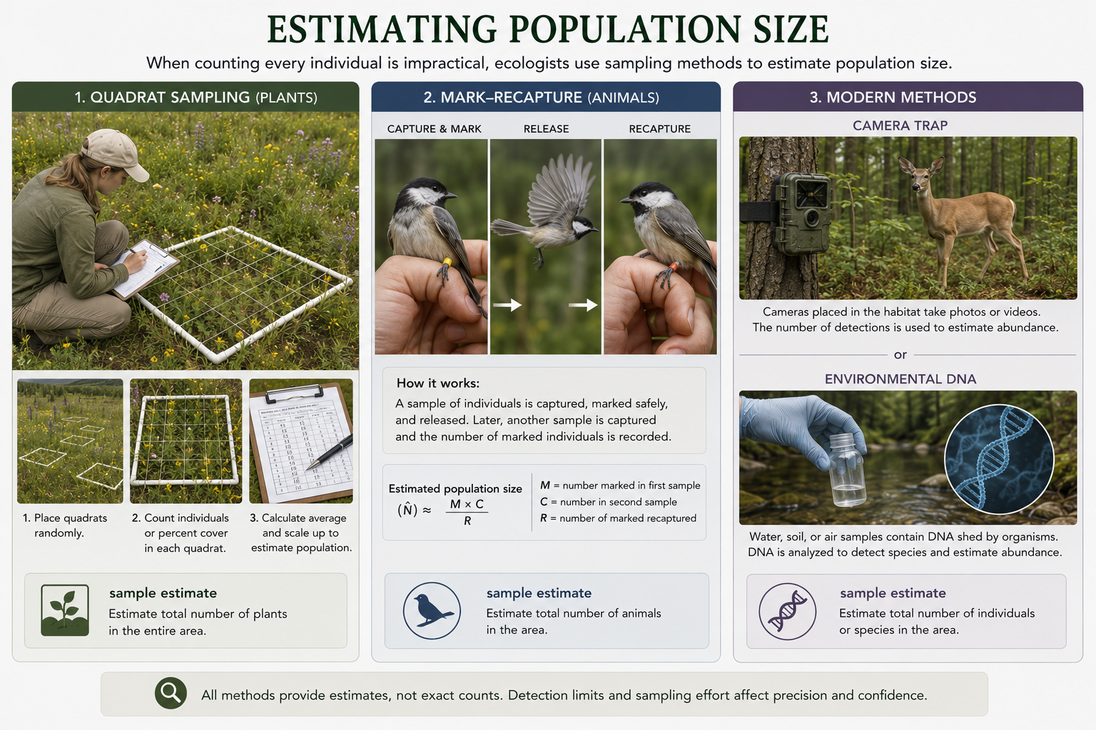
Figure 4. Estimating Population Size. Ecologists often estimate population size using sampling methods such as quadrats, mark-recapture, camera traps, acoustic monitoring, environmental DNA, or repeated surveys. Each method has strengths and limits.
Dispersion Patterns
Individuals in a population are not always spread evenly across space. Dispersion describes how individuals are distributed within an area. In a clumped dispersion, individuals occur in groups. This is common when resources are patchy, when animals form herds or schools, or when offspring remain near parents. Fish may show clumped dispersion because they school for protection. In a uniform dispersion, individuals are spaced more evenly. This often occurs when individuals defend territories or compete strongly for space, water, light, or nutrients. For example, desert shrubs may show uniform spacing because each shrub uses water from the surrounding soil and limits the success of nearby seedlings. In a random dispersion, individuals are distributed unpredictably, usually when resources are widespread and individuals do not strongly attract or repel one another. Trees with wind-dispersed seeds may appear more random if seeds land unpredictably and resources are not strongly patchy. Dispersion patterns help ecologists understand behavior, resource availability, competition, reproduction, and habitat structure. Dispersion is one way population ecologists connect spatial patterns to ecological processes.
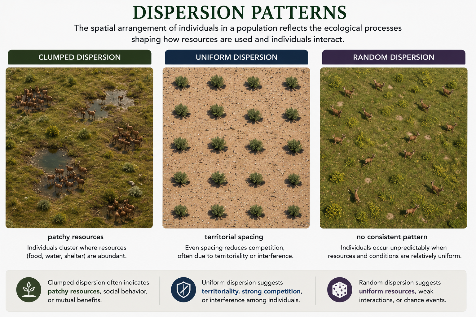
Figure 5. Dispersion Patterns. Dispersion describes how individuals are distributed within an area. Clumped, uniform, and random patterns can reveal resource distribution, competition, territoriality, reproduction, social behavior, and habitat structure.
Survivorship Curves
A survivorship curve is a graph that shows the proportion of individuals in a population that survive to different ages. Ecologists often describe three general survivorship patterns. Type I survivorship occurs when most individuals survive through early and middle life, with mortality increasing later in life. Humans and many large mammals often show this pattern. Type II survivorship occurs when the chance of death is relatively constant throughout life. Some birds, reptiles, and small mammals approximate this pattern. Type III survivorship occurs when many individuals die early in life, but those that survive the earliest stages may live much longer. Many plants, fish, marine invertebrates, and insects show this pattern. For example, an oak tree may produce thousands of acorns, but only a small number become seedlings, and even fewer grow into mature trees. Survivorship curves help ecologists compare life histories and understand when mortality is strongest during an organism’s life. These curves are simplified models, so not every species fits perfectly into one category. Still, they are useful because they show that species differ greatly in when death is most likely to occur.
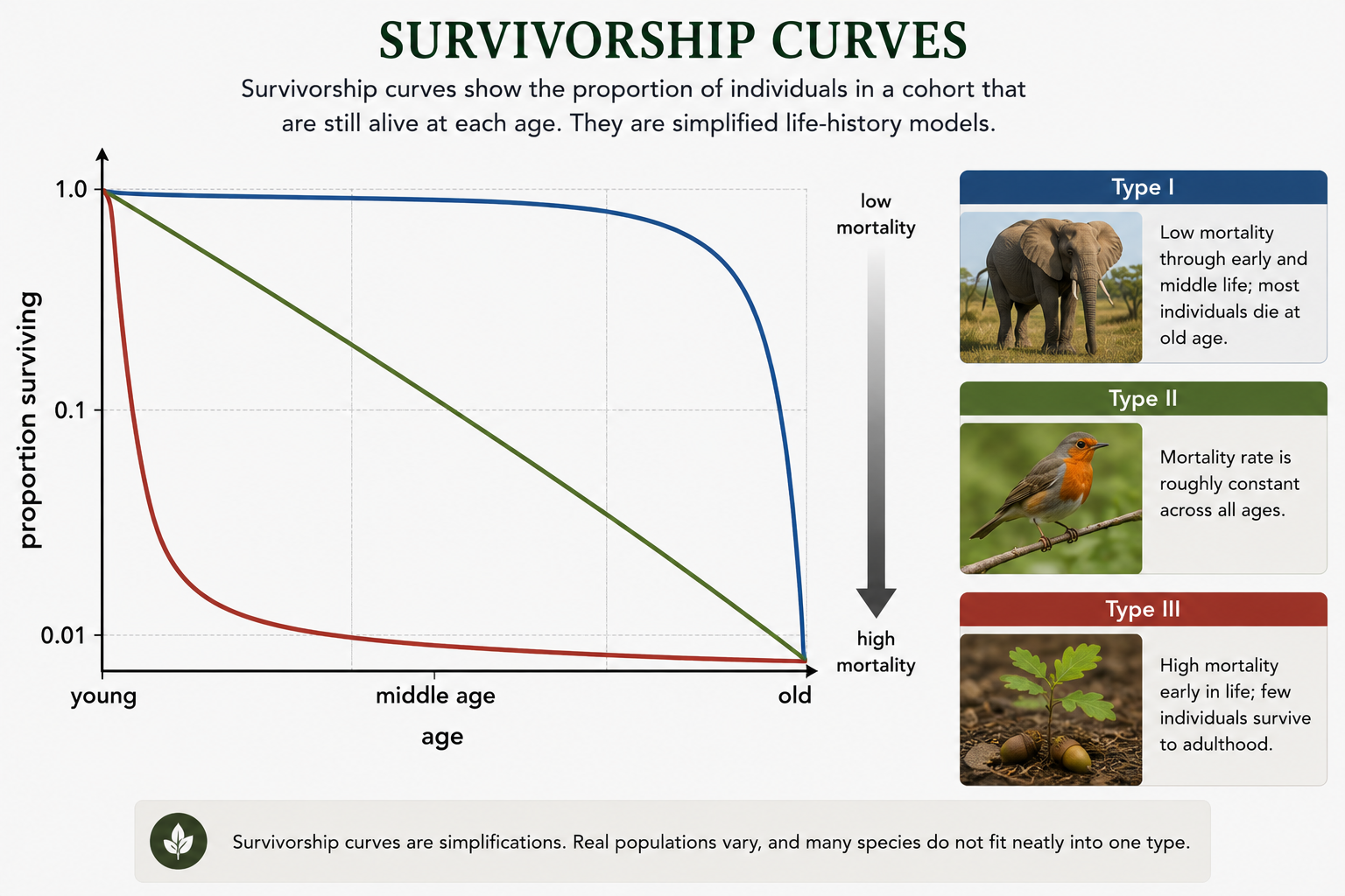
Figure 6. Survivorship Curves. Survivorship curves show the proportion of individuals that survive to different ages. Type I species have low early mortality, Type II species have relatively constant mortality, and Type III species have high early mortality.
Fecundity and Reproductive Investment
Fecundity is the reproductive output of an organism or population, often measured as the number of offspring produced by females at a particular age. Some species produce many offspring at once but provide little parental care. Many fish, insects, amphibians, and plants follow this pattern. Other species produce fewer offspring but invest more energy into each one. Elephants, whales, humans, and many birds are examples of species with lower offspring number but higher parental investment. Neither strategy is automatically better. Producing many offspring can be successful when early mortality is high and parental care is limited. Producing fewer offspring can be successful when survival improves because parents provide protection, nutrition, learning, or care. Population ecologists use fecundity and survivorship together to estimate how quickly populations may grow or decline. A species with high fecundity may still grow slowly if most offspring die before reproducing. A species with low fecundity may maintain a stable population if offspring survival is high. Reproductive output only makes sense when considered together with survival.
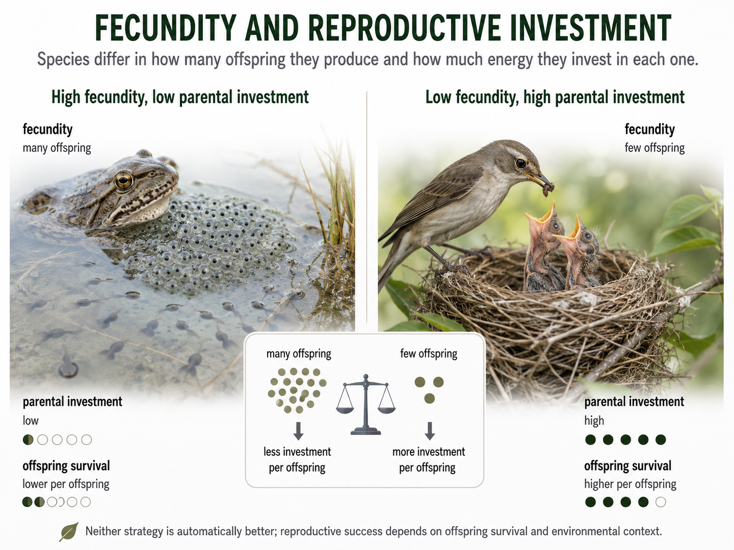
Figure 7. Fecundity and Reproductive Investment. Fecundity is reproductive output, often measured as the number of offspring produced. Some species produce many offspring with little care, while others produce fewer offspring and invest more heavily in each one.
Life Tables
A life table is a summary of survival and reproduction at different ages or life stages. Life tables help ecologists estimate how many individuals survive from one age class to the next and how many offspring individuals produce at each stage. For example, a life table for a plant might track seeds, seedlings, juveniles, reproductive adults, and older adults. A life table for an animal might track newborns, juveniles, young adults, mature adults, and old adults. Life tables are useful because population growth depends not only on how many individuals are alive, but also on which ages or life stages are present. A population with many reproductive adults may grow quickly. A population with mostly old individuals and few young may decline. Life tables connect survivorship, fecundity, and age structure into one demographic picture. They are especially useful in conservation because they can identify vulnerable life stages. For example, if a turtle population produces many eggs but few hatchlings survive, protecting nests may matter most. If many juveniles survive but few adults reproduce, protecting adult habitat may be more important.
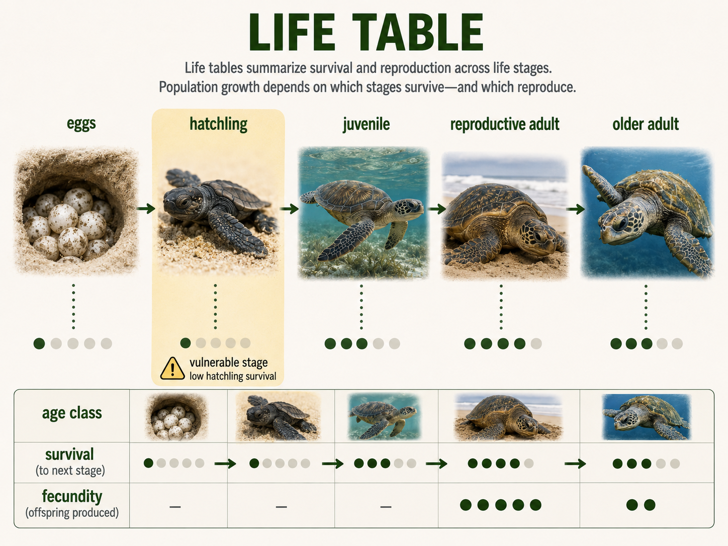
Figure 8. Life Tables. A life table summarizes survival and reproduction at different ages or life stages. Life tables help ecologists understand which stages contribute most to population growth or decline.
Fitness Trade-Offs
Fitness is an organism’s ability to survive and reproduce in a particular environment. Because energy and resources are limited, organisms face trade-offs. They cannot maximize every possible trait at the same time. Energy used for reproduction cannot also be used for growth, immune defense, repair, escape, or long-term survival. A bird that lays a very large clutch of eggs may produce many offspring in one season, but it may also reduce its own chance of surviving to the next year because feeding many chicks requires more energy. A bird that lays fewer eggs may have a better chance of surviving, but it produces fewer offspring that season. Many organisms fall somewhere between these extremes, balancing reproduction and survival depending on their environment. Trade-offs are central to population ecology because they explain why different species have different life history strategies. A plant may invest heavily in seeds, roots, leaves, defense chemicals, or rapid growth, but it cannot invest maximally in all of them at once. Natural selection shapes these trade-offs over generations.
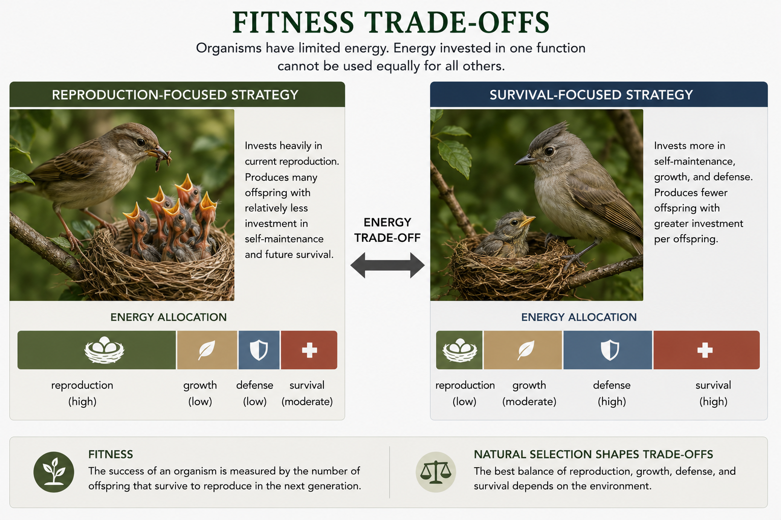
Figure 9. Fitness Trade-Offs. Because energy and resources are limited, organisms cannot maximize every trait at the same time. Investment in reproduction, growth, defense, repair, or survival often involves trade-offs.
Life History Strategies
A life history strategy is the pattern of growth, reproduction, survival, and parental investment that characterizes a species. Species with fast life histories often mature quickly, reproduce early, produce many offspring, and have shorter lifespans. Species with slow life histories often mature later, reproduce more slowly, produce fewer offspring, invest more in each offspring, and live longer. These contrasts are often described as either r-selected or K-selected species. In this model, r-selected species are associated with rapid population growth, high fecundity, small body size, short lifespans, and unstable environments. K-selected species are associated with slower growth, stronger competitive ability, larger body size, longer lifespans, and populations near carrying capacity. This model is useful as an introduction, but real life histories are more complex. Modern ecologists treat life history traits as a continuum shaped by natural selection, environment, mortality, resource availability, and evolutionary history. For example, a species may mature quickly but still provide parental care, or it may live long but produce many small offspring. The r/K model is best used as a starting framework, not a rigid classification system.
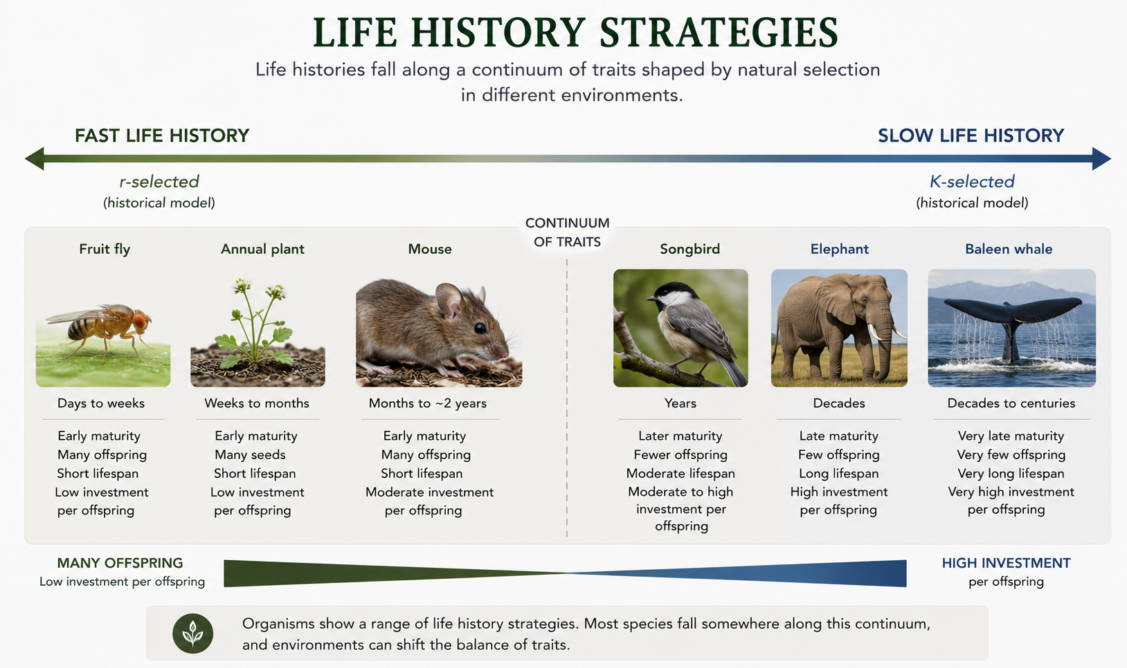
Figure 10. Life History Strategies. Life history strategies describe patterns of growth, reproduction, survival, and parental investment. Fast and slow life histories form a continuum shaped by natural selection, environment, mortality, resources, and evolutionary history.
Population Growth Rate
Population growth rate describes how quickly a population changes over time. Ecologists often use r to represent the per capita rate of increase. A population grows when births exceed deaths, declines when deaths exceed births, and remains stable when births and deaths are balanced. In simple models that ignore immigration and emigration, r can be described as the birth rate minus the death rate. If r is positive, the population increases. If r is negative, the population decreases. If r is zero, the population is not changing in size. In real populations, r can change through time because birth rates, death rates, resource availability, predation, disease, weather, and human impacts also change. The growth rate of a population is one of the most important measurements in ecology because it helps scientists predict whether a population is expanding, shrinking, or remaining stable. Growth rate can be measured over short periods, such as a breeding season, or longer periods, such as decades. Ecologists must be careful because short-term growth does not always predict long-term trends.
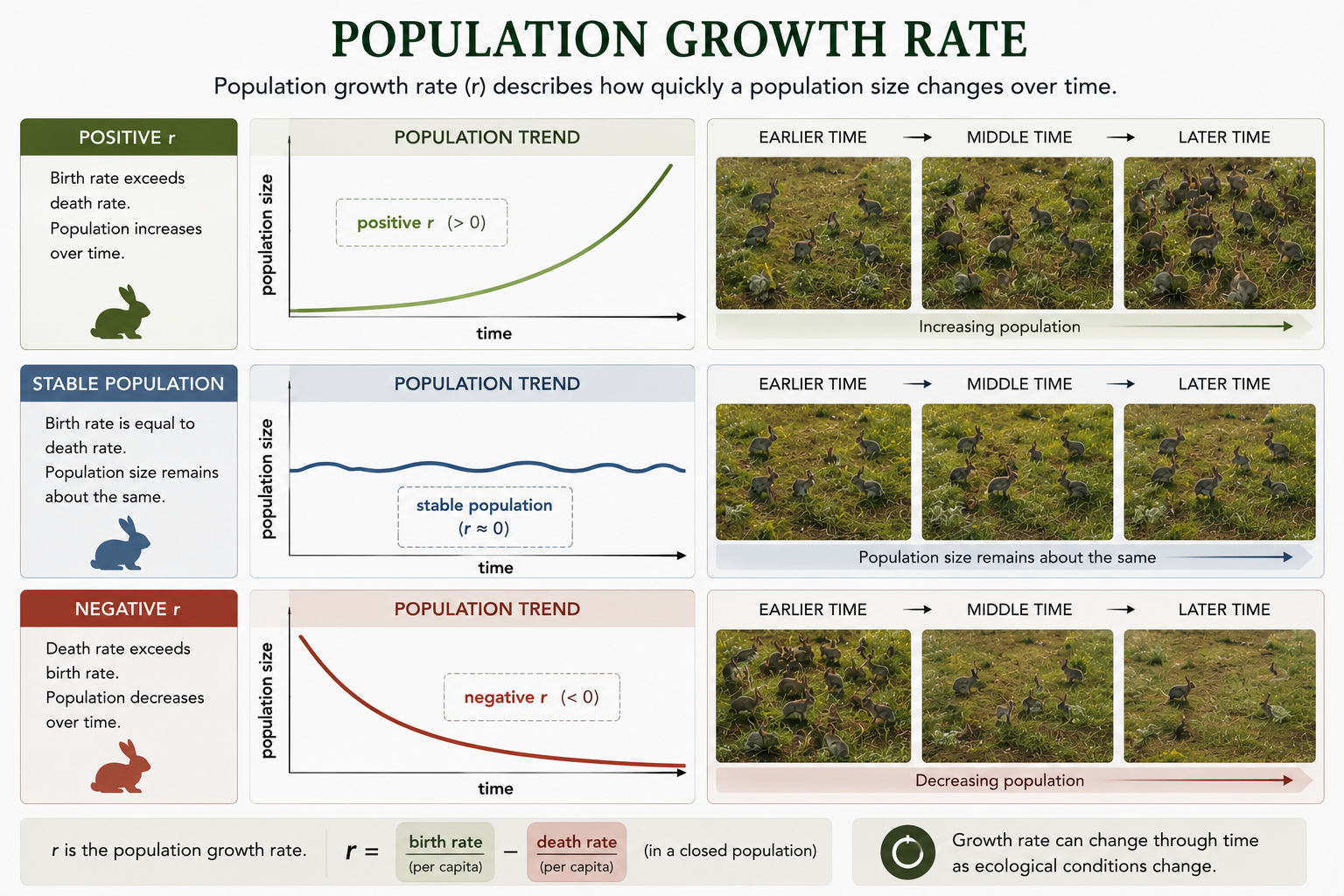
Figure 11. Population Growth Rate. Population growth rate describes how quickly a population changes over time. In simple closed-population models, growth depends on the balance between birth rate and death rate.
Exponential Growth
Exponential growth occurs when a population increases by the same proportion during each time interval. In this model, the population growth rate does not decline as population size increases. Exponential growth can be described as: dN/dt = rN, where N is population size, r is the per capita growth rate, and dN/dt is the change in population size through time. This kind of growth produces a J-shaped curve. For example, if a population doubles each generation, 2 individuals become 4, 4 become 8, 8 become 16, and 16 become 32. Exponential growth can occur when a population enters a new habitat, when resources are abundant, when predators or competitors are absent, or when a population recovers after a severe disturbance. However, exponential growth cannot continue forever in a finite environment. Eventually, resources become limited, waste accumulates, disease spreads more easily, or competition increases. At that point, population growth slows. Exponential growth is therefore most useful for understanding early growth under favorable conditions, not permanent growth in a real ecosystem.
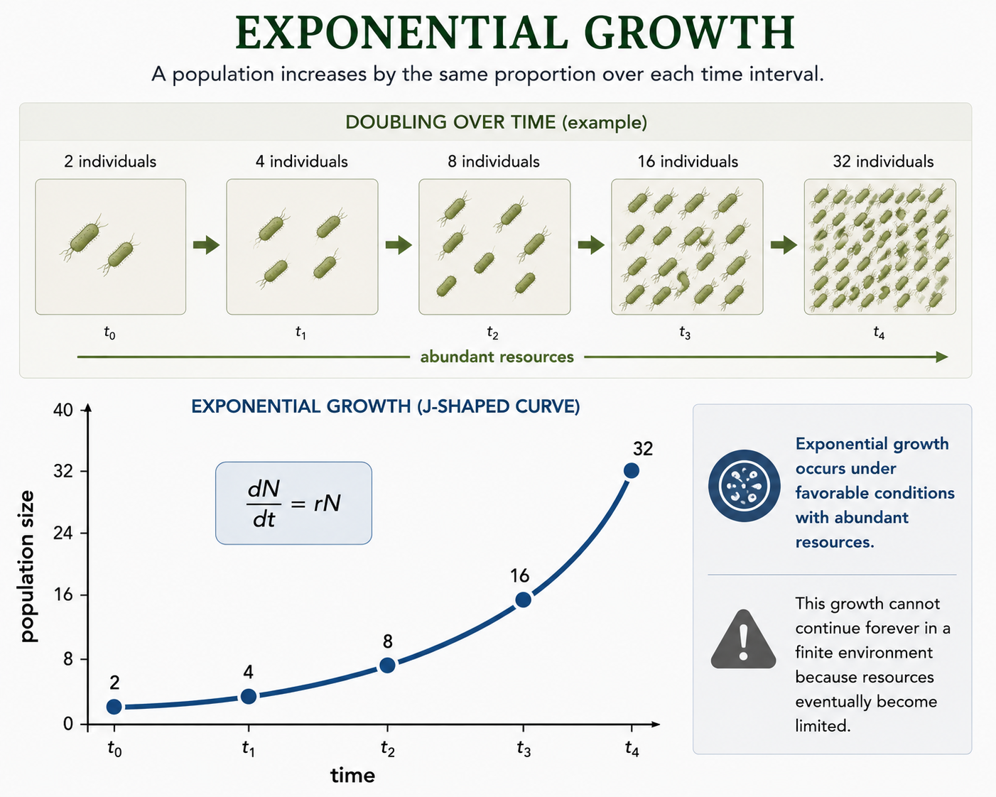
Figure 12. Exponential Growth. Exponential growth occurs when a population increases by the same proportion during each time interval. This produces a J-shaped curve and is most likely under favorable conditions with abundant resources.
Density-Independent and Density-Dependent Growth
Population growth depends on how many individuals are born and how many die. Some factors affect populations no matter how large or small the population is. These are called density-independent factors. Examples include droughts, floods, fires, freezes, hurricanes, pollution, and habitat destruction. These events can reduce a population even when the population is not crowded. Other factors depend on how crowded the population is. These are called density-dependent factors. As a population gets larger, individuals may compete more for food, water, space, light, mates, or nesting sites. Crowding can also make disease, parasites, and predators more important. For example, disease can spread more easily in a crowded population than in a spread-out population. Density-dependent factors help explain why populations usually do not grow forever. When a population is small, resources may be easy to find, so the population can grow quickly. As the population gets closer to the carrying capacity, resources become more limited and growth slows down. The carrying capacity is the largest population size an environment can support over time. Both types of factors affect population size. Density-independent factors often cause sudden changes, such as population crashes after a storm or drought. Density-dependent factors usually slow population growth as the population becomes more crowded.
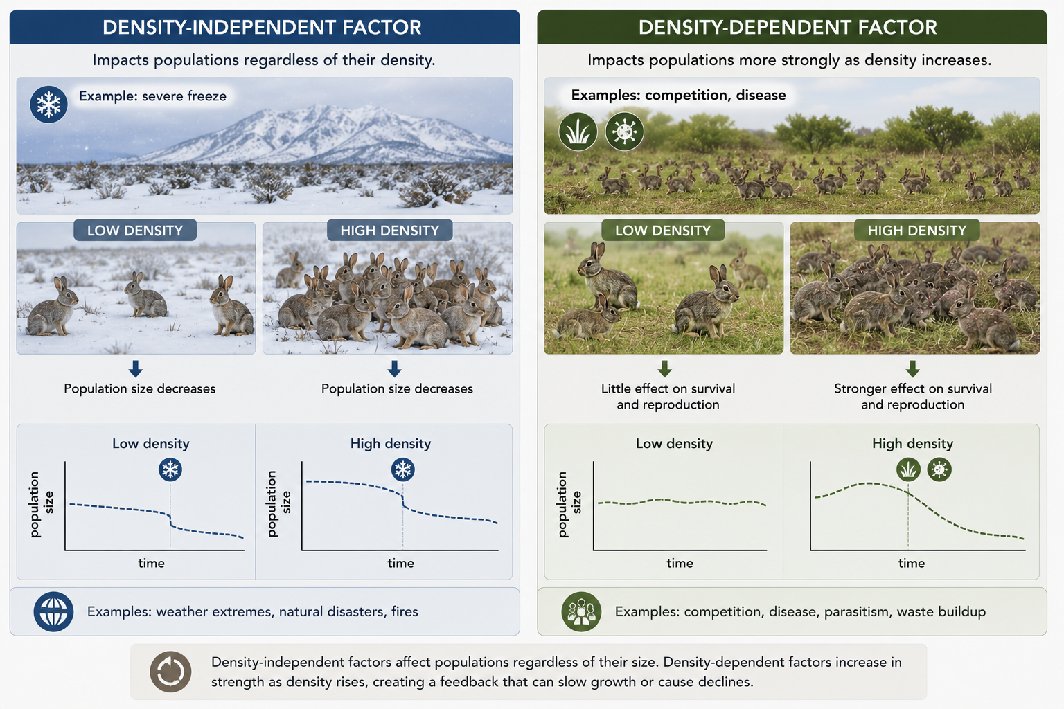
Figure 13. Density-Independent and Density-Dependent Growth. Density-independent factors affect populations regardless of crowding, while density-dependent factors become stronger as population density increases. Density-dependent feedback can slow population growth as populations become crowded.
Carrying Capacity
Carrying capacity is not a fixed number that stays the same forever. It varies among species, habitats, seasons, years, and environmental conditions. A wet year may increase plant growth and raise the carrying capacity for herbivores. A drought may reduce food and water, lowering carrying capacity. A habitat with abundant resources and low predation may support more individuals than a habitat with limited resources and high predation. Human activity can also change carrying capacity by adding resources, removing predators, fragmenting habitat, polluting ecosystems, or altering climate. Carrying capacity is best understood as a dynamic ecological limit, not a permanent ceiling. Populations may fluctuate around K, overshoot it, crash below it, and recover again depending on conditions. Carrying capacity also depends on which resource is most limiting. A habitat may have plenty of space but too little food, plenty of food but too few nesting sites, or suitable habitat but too much predation. The limiting factor determines how many individuals the environment can actually support.
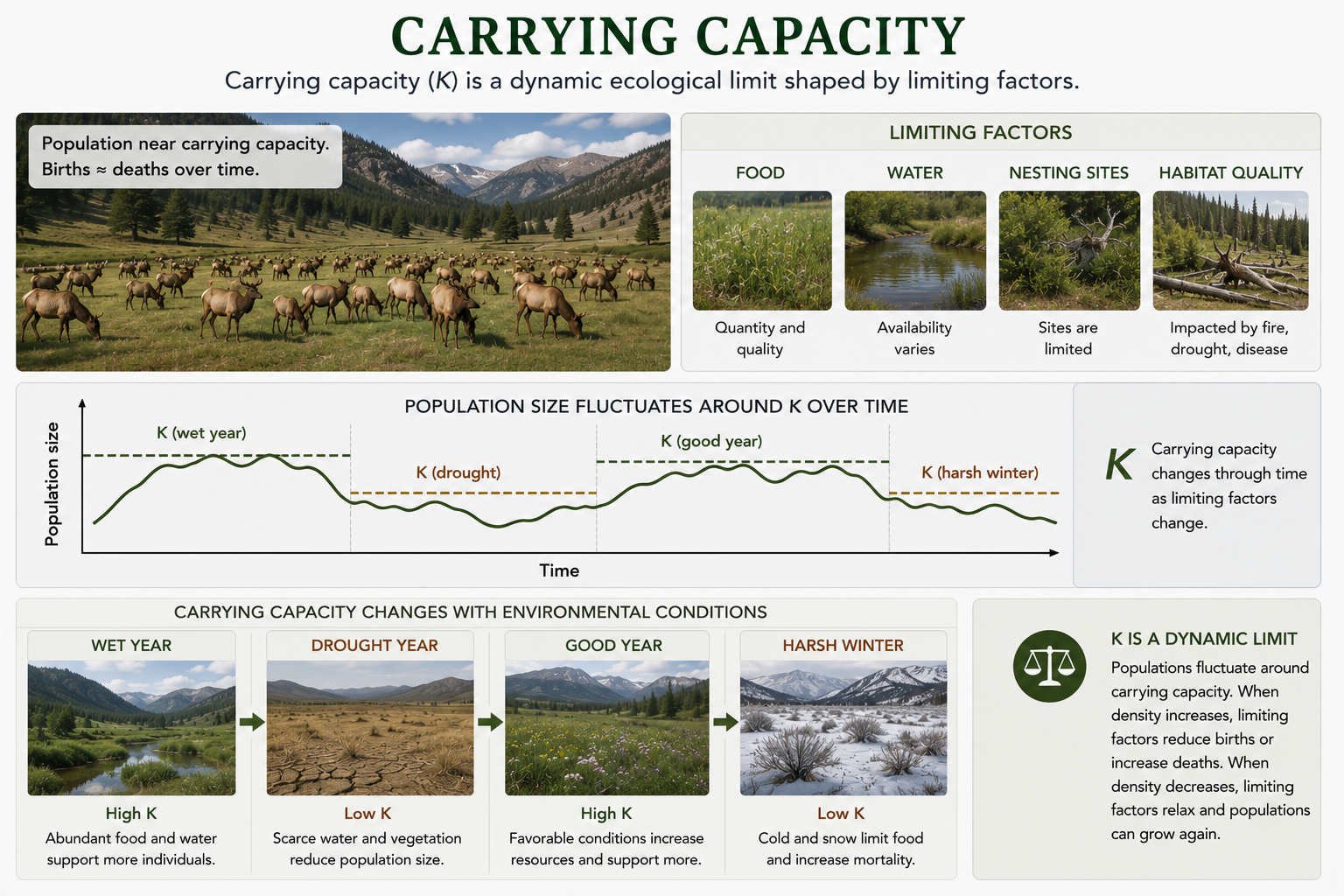
Figure 14. Carrying Capacity. Carrying capacity is the number of individuals an environment can support under particular conditions. It changes with resources, habitat quality, seasons, predation, climate, and human activity.
Density Dependence in Real Life
Density dependence is easy to see in gardens, forests, wildlife populations, and disease outbreaks. In a garden, seedlings planted too closely compete for light, water, nutrients, and space. If the gardener does not thin them, there may be many plants, but each plant may grow poorly and produce less food. In forests, dense seedlings compete strongly, and many die before reaching maturity. In animal populations, high density can increase competition for food, nesting sites, or mates. High density can also increase disease transmission because individuals come into contact more often. Density-dependent factors often regulate populations by reducing birth rates, increasing death rates, or encouraging emigration when populations become crowded. Density dependence can also influence body condition and reproduction. Crowded animals may be smaller, produce fewer offspring, or reproduce later. Crowded plants may grow tall and thin as they compete for light but produce fewer seeds. These effects show that population density can influence both the number and quality of individuals in a population.
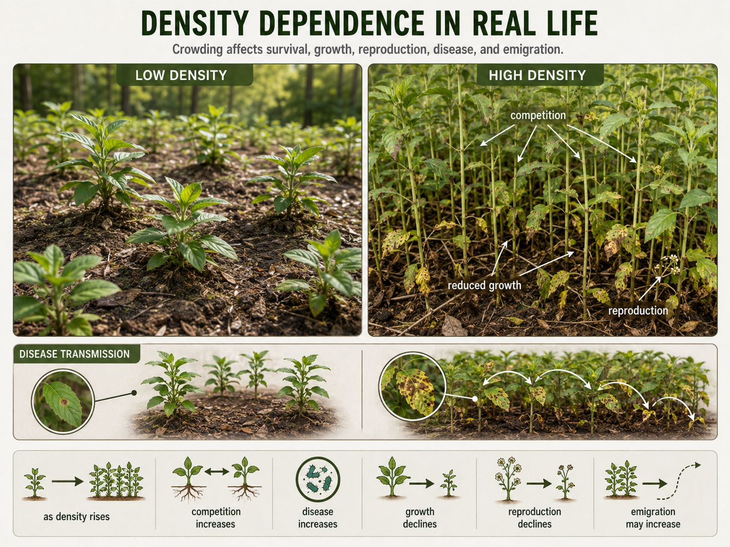
Figure 15. Density Dependence in Real Life. Density-dependent factors become stronger as populations become crowded. High density can increase competition, disease transmission, stress, emigration, and reduced growth or reproduction.
Allee Effects
An Allee effect occurs when population growth is reduced at very low population density. This is the opposite of what simple density-dependence models often emphasize. In many cases, low density reduces competition and should help individuals survive. However, populations can become so sparse that individuals have trouble finding mates, cooperating, defending against predators, or maintaining social structure. For example, some animals need a group to hunt, raise young, or detect predators effectively. Some plants may reproduce poorly if individuals are too far apart for pollinators to move pollen between them. Allee effects are especially important in conservation biology because small populations may decline even when resources are available. Once a population falls below a critical threshold, recovery can become difficult without protection, habitat restoration, or reintroduction of individuals.
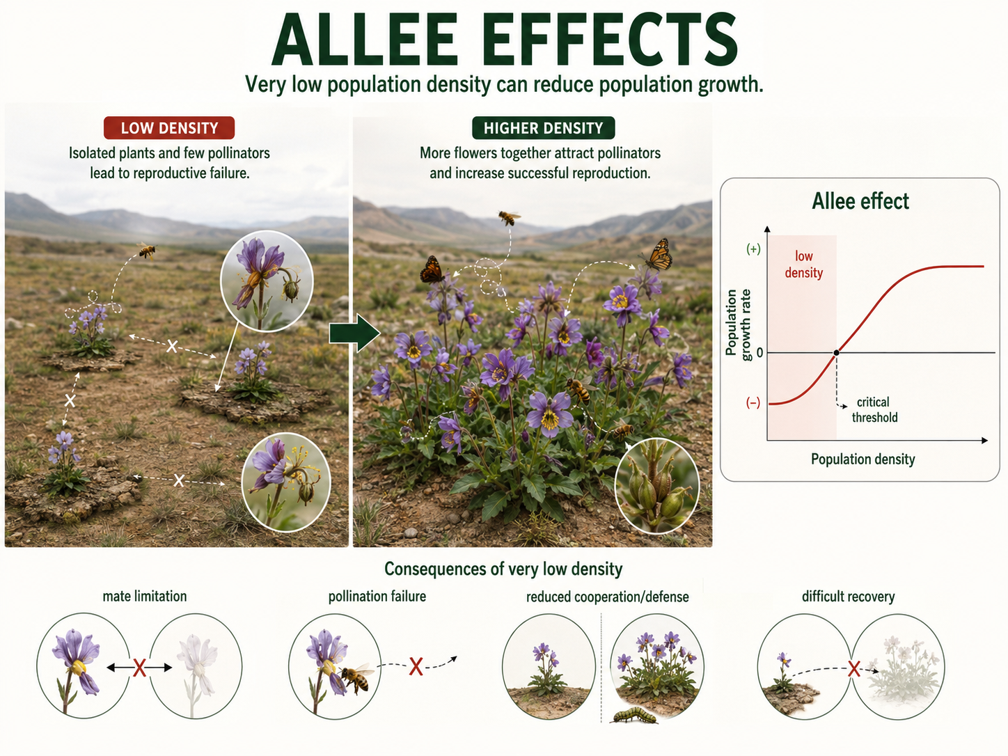
Figure 16. Allee Effects. An Allee effect occurs when population growth is reduced at very low density. Sparse populations may struggle to find mates, cooperate, defend against predators, maintain social structure, or reproduce successfully.
Overshoot and Population Crashes
Sometimes a population can overshoot, or grow beyond the carrying capacity of its environment. Overshoot can happen when resources appear abundant for a short time, when there is a delay before density-dependent effects are felt, or when a population is introduced into a new habitat without its usual predators or competitors. After overshoot, the population may experience a crash, a rapid decline in population size. Crashes can occur when food is depleted, disease spreads, waste accumulates, or environmental conditions change. Overshoot and crash dynamics are common in some natural populations and are especially important in conservation, pest management, and human resource use. They remind us that population growth can have delayed consequences. A population may appear successful for a time, even as it is using resources faster than those resources can recover. When the shortage finally appears, the decline may be sudden.
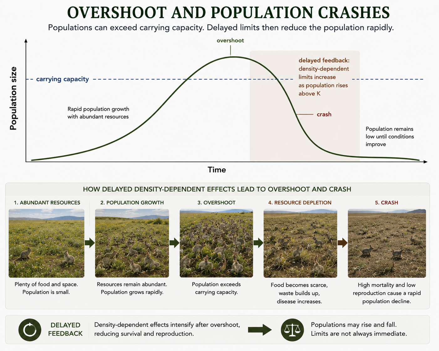
Figure 17. Overshoot and Population Crashes. Overshoot occurs when a population grows beyond carrying capacity. If resources are depleted or density-dependent effects appear after a delay, the population may experience a rapid crash.
Population Cycles
Some populations rise and fall in repeating or semi-repeating cycles. Population cycles can occur when predator and prey populations influence each other, when food availability changes regularly, or when climate patterns affect survival and reproduction. In a predator-prey cycle, prey populations may increase when food is abundant and predation is low. Predator populations may then increase because more prey are available. As predators become more abundant, prey decline. Later, predators may decline because there is less food, allowing prey to increase again. Real population cycles are rarely perfectly smooth because weather, disease, migration, and habitat changes also matter. Still, cycles show that population size is often dynamic rather than constant. Populations may fluctuate naturally even in the absence of human disturbance.
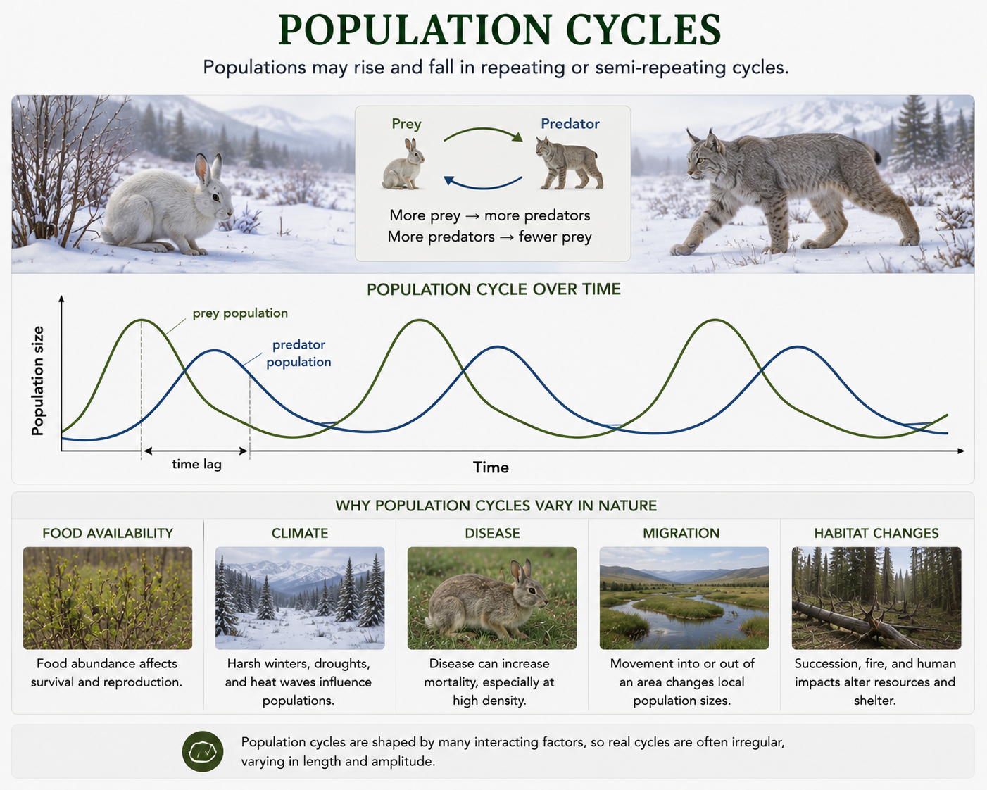
Figure 18. Population Cycles. Some populations rise and fall in repeating or semi-repeating cycles. Predator-prey interactions, food availability, climate, disease, migration, and habitat conditions can all contribute to these fluctuations.
Metapopulations
A metapopulation is a group of local populations connected by movement among habitat patches. Instead of thinking about one large continuous population, metapopulation ecology studies many smaller populations across a landscape. Some patches may contain thriving populations, some may contain small declining populations, and some may be temporarily empty. Local populations can go extinct, and empty patches can later be recolonized by individuals from other patches. This balance between local extinction and recolonization is central to metapopulation dynamics. Metapopulations are especially important in fragmented habitats, where roads, farms, cities, or other barriers divide suitable habitat into isolated patches. Conservation biologists use metapopulation theory to design wildlife corridors, protect habitat networks, and reduce the risk that isolated populations will disappear permanently. A species may survive across a region not because every patch remains occupied forever, but because movement among patches continually rescues or recolonizes local populations.
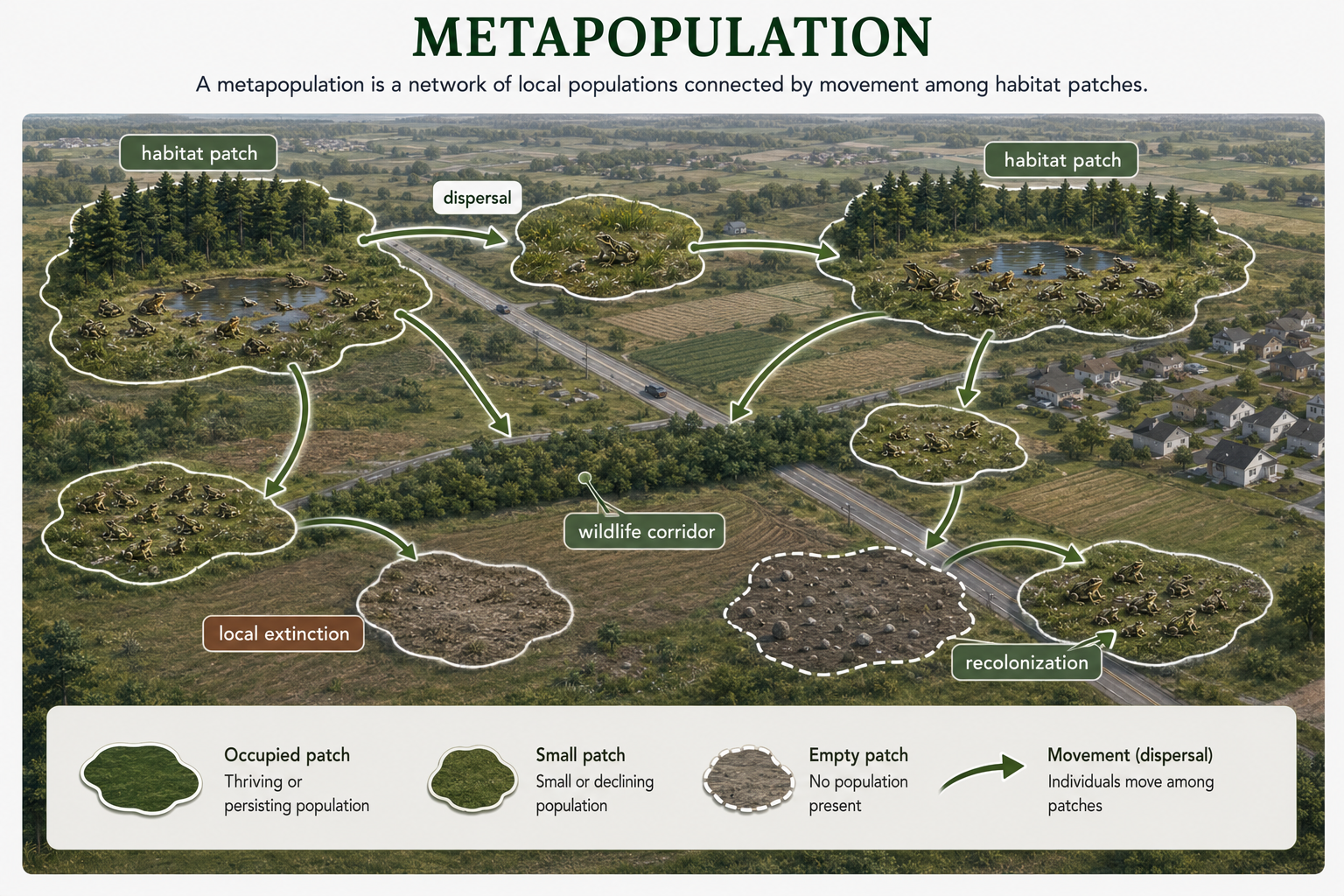
Figure 19. Metapopulations. A metapopulation is a group of local populations connected by movement among habitat patches. Local populations may go extinct, empty patches may be recolonized, and dispersal can help the species persist across a region.
Source and Sink Populations
Within a metapopulation, some habitat patches are better than others. A source population lives in a high-quality habitat where birth rates are greater than death rates, producing extra individuals that can disperse to other areas. A sink population lives in a lower-quality habitat where death rates are greater than birth rates, so the population may persist only because immigrants arrive from source populations. Source and sink dynamics are important because a population may appear stable in a poor habitat even though it cannot sustain itself without immigration. For conservation, this means that protecting only the places where a species is seen may not be enough. Ecologists must identify which habitats actually produce enough surviving offspring to support the broader population. A sink habitat can be misleading because individuals are present, but the habitat may not contribute to long-term population growth. Protecting source habitats is often essential for keeping the whole metapopulation alive.
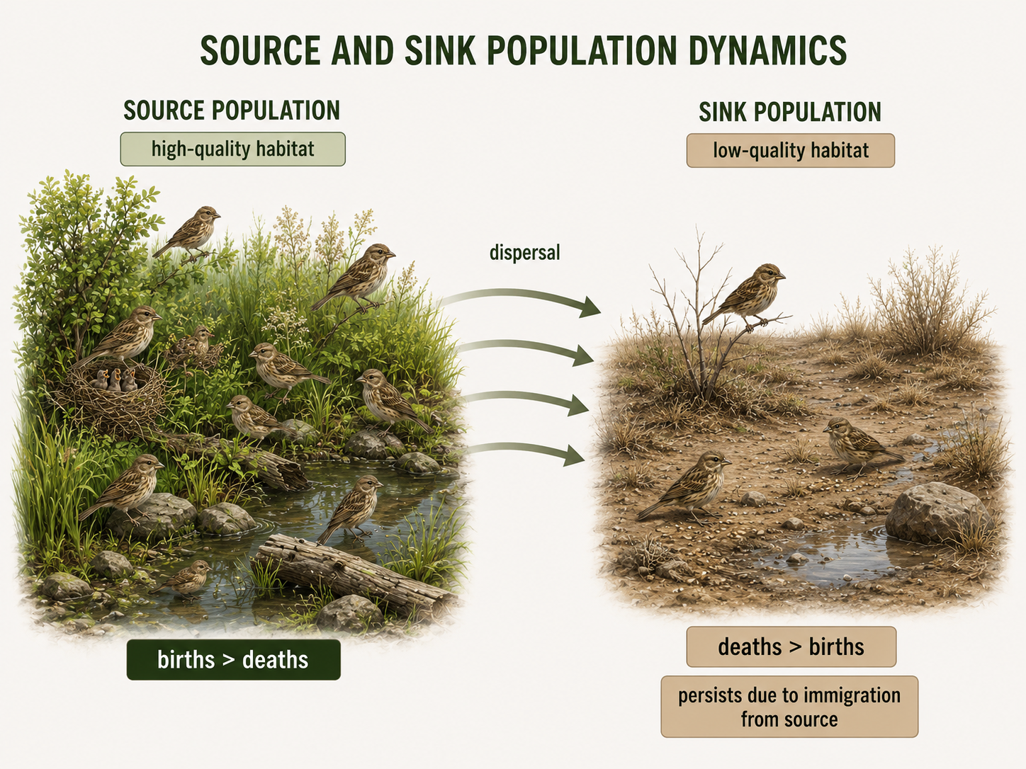
Figure 20. Source and Sink Populations. Source populations live in high-quality habitats where births exceed deaths and surplus individuals disperse. Sink populations live in lower-quality habitats where deaths exceed births and persistence may depend on immigration.
Age Structure
Age structure is the proportion of individuals in a population found in each age group or life stage. Age structure matters because individuals of different ages contribute differently to population growth. A population with many young individuals may grow rapidly if those individuals survive to reproductive age. A population with many reproductive adults may be stable or expanding. A population made mostly of older individuals and few young may decline in the future. In plants, ecologists may study seed banks, seedlings, saplings, reproductive adults, and older adults. After a tree falls and creates a forest gap, many seedlings may establish because light reaches the forest floor. Over time, many seedlings die, some become saplings, and only a few become mature adults. By studying age structure, ecologists can predict future population trends before population size changes become obvious. Age structure is especially important for long-lived species because population decline may be hidden for years if adults remain alive but few young survive to replace them.
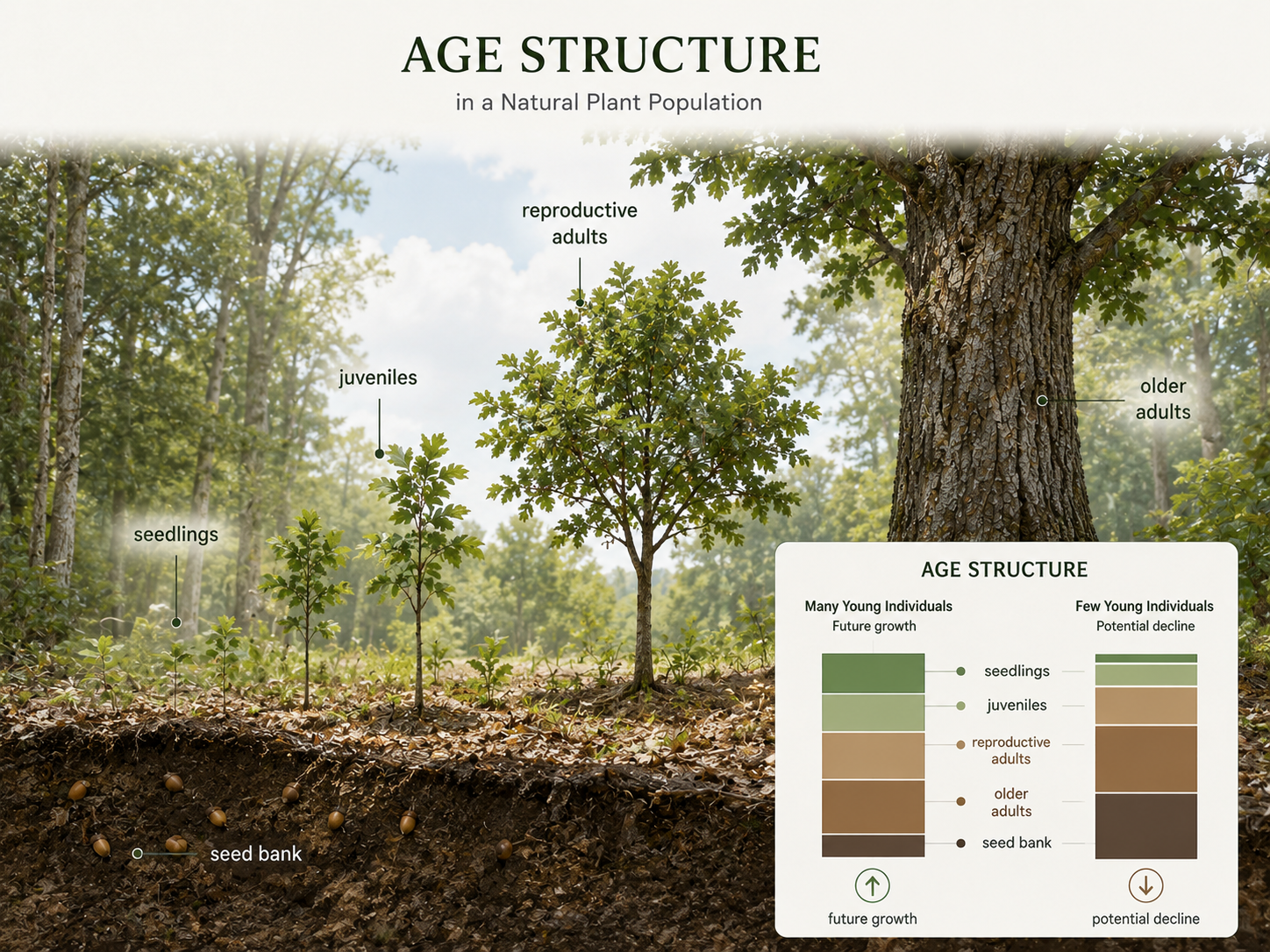
Figure 21. Age Structure. Age structure describes the proportion of individuals in different age groups or life stages. It helps ecologists predict population trends before changes in total population size become obvious.
Human Age Structure
Human populations also have age structures, often shown as population pyramids. A country with many children and young adults has a broad-based age structure and may grow rapidly as those young people reach reproductive age. A country with a more even distribution across age groups may grow slowly or remain stable. A country with many older adults and fewer young people may face population aging and possible future decline. Age structure reflects birth rates, death rates, life expectancy, migration, health care, economic conditions, education, and social factors. In many high-income countries, birth rates are low and life expectancy is high, producing older population structures. In many lower-income or rapidly growing countries, younger age structures are more common, though patterns vary widely. Human age structure is important because it affects schools, jobs, health care, retirement systems, housing, and future population growth. A young population may need more schools and job creation, while an aging population may need more health care workers, elder care, and retirement support.
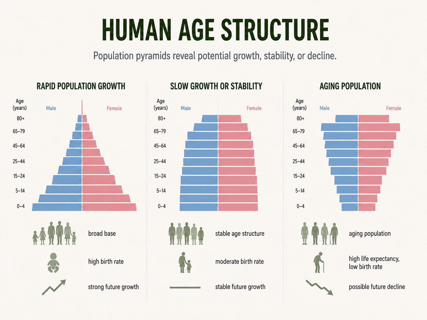
Figure 22. Human Age Structure. Human age structure is often shown with population pyramids. Broad-based age structures suggest potential rapid growth, rectangular structures suggest slower growth or stability, and top-heavy structures suggest aging and possible future decline.
History of Human Population Growth
For most of human history, the human population grew very slowly. Birth rates were often high, but death rates were also high because of disease, famine, poor sanitation, limited medical care, high infant mortality, and unreliable food supplies. In population ecology, this means human population size was strongly limited by survival and resource availability. Even when families had many children, many children did not survive to adulthood, so the total population increased only gradually. This pattern changed as humans developed agriculture, food storage, sanitation systems, vaccination, antibiotics, modern medicine, and public health programs. These advances lowered death rates, especially among infants and children. When more people survived but birth rates remained high, the global population began to grow rapidly. This rapid increase was especially strong during the last few centuries and represents one of the most important demographic changes in human history. Today, the human population is over 8 billion. The United Nations estimates that the world population will continue growing for several more decades, reaching about 10.3 billion in the mid-2080s before declining slightly by 2100. This means the population is still increasing, but the growth rate is slowing. From a population ecology perspective, human population growth is no longer simple exponential growth. It is shaped by fertility rates, survivorship, age structure, education, health care, economic development, resource use, and the ecological limits of the planet.
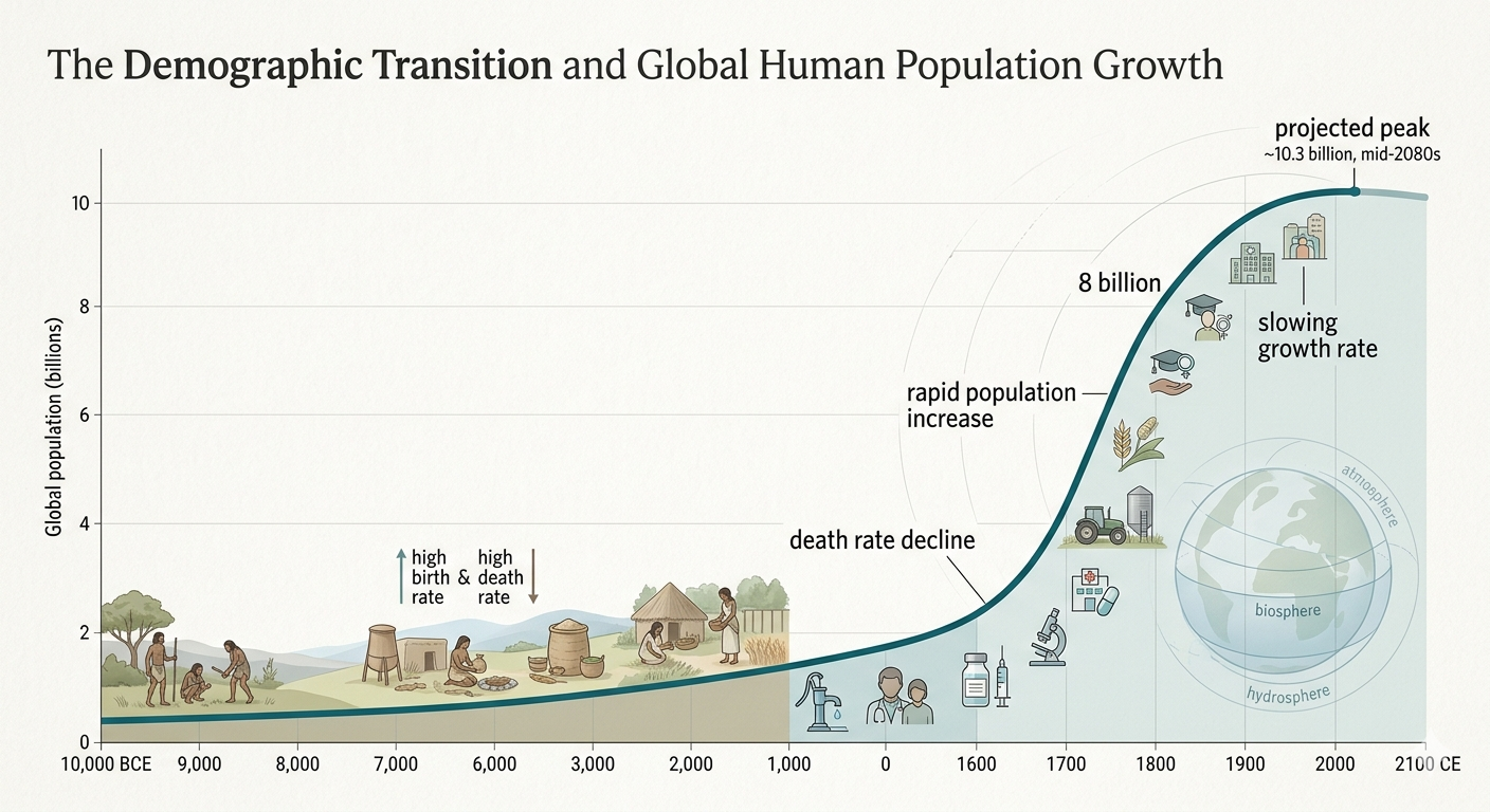
Figure 23. History of Human Population Growth. Human population growth was slow for most of history because high birth rates were balanced by high death rates. Improvements in agriculture, sanitation, vaccination, antibiotics, medicine, and public health lowered death rates and caused rapid growth, but global growth is now slowing as fertility rates decline.
Human Carrying Capacity
Today, the world population is over 8 billion. The United Nations projects that it may reach about 10.3 billion in the mid-2080s before declining slightly by 2100. This means the human population is still growing, but the growth rate is slowing. Population ecology helps explain this pattern. Human population growth depends on birth rates, death rates, fertility, survivorship, age structure, and carrying capacity. In many countries, birth rates have declined because of education, health care, urbanization, contraception, economic change, and shifting social expectations. However, countries with many young people may continue growing for decades because many individuals are entering their reproductive years. The carrying capacity of Earth for humans is difficult to estimate because humans are not limited by resources in exactly the same way as many other species. Technology, agriculture, trade, medicine, and energy use can increase the number of people Earth can support. However, these advances also have environmental costs. Human carrying capacity depends not only on food and water, but also on soil, freshwater, energy, biodiversity, climate stability, pollution, waste production, consumption rates, and how resources are distributed. For humans, the question is not only “How many people can Earth hold?” The better question is “How many people can Earth support at a good quality of life without damaging the natural systems that support life?” A planet with billions of people using resources carefully is very different from a planet with billions of people consuming at very high levels. Human carrying capacity can be raised by innovation, efficiency, conservation, and fair resource use, but it can also be lowered by soil degradation, freshwater scarcity, climate change, habitat loss, pollution, and unequal access to resources.
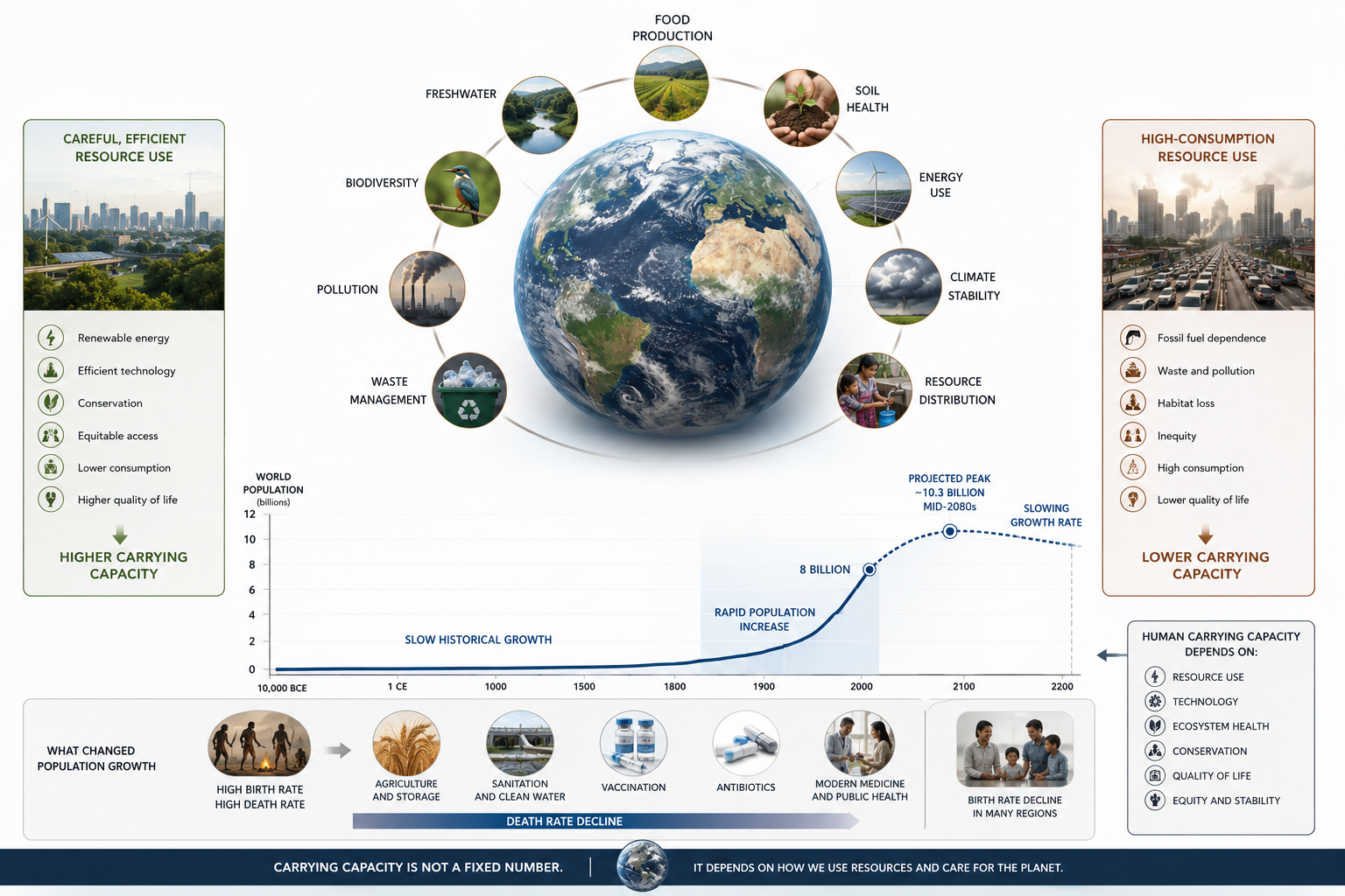
Figure 24. Human Population Growth and Carrying Capacity. The human population is still growing, but the growth rate is slowing as fertility declines in many regions. Human carrying capacity is difficult to estimate because it depends on food, water, soil, energy, biodiversity, climate stability, pollution, waste, consumption rates, technology, conservation, and resource distribution.
Predicted Human Population Growth, Decline, and Environmental Consequences
The human population is still growing, but it is growing more slowly than it did in the past. Humans are not expected to keep growing exponentially forever because birth rates are declining in many parts of the world. One likely future is gradual population decline in some countries. This is already happening, or beginning to happen, in places with low fertility rates and aging populations. In these countries, deaths may eventually outnumber births, causing the population to slowly shrink over time. Gradual population decline is different from a population crash. A decline usually happens slowly and is often caused by social changes, such as smaller family sizes, delayed reproduction, urbanization, education, and economic pressures. A population crash happens much more quickly. In population ecology, a crash often occurs after a population exceeds the resources available to support it, leading to a rapid drop in population size. From a population ecology perspective, the main risk is overshoot. Overshoot happens when a population uses resources faster than they can be replaced or damages the environment faster than it can recover. For humans, this could involve overusing freshwater, degrading soil, clearing forests, overfishing, polluting ecosystems, or increasing climate stress. Technology can reduce some limits, but it cannot remove ecological limits completely. The future will likely be uneven: some regions will continue growing, some will shrink and age, and some may face serious environmental, economic, and social stress.
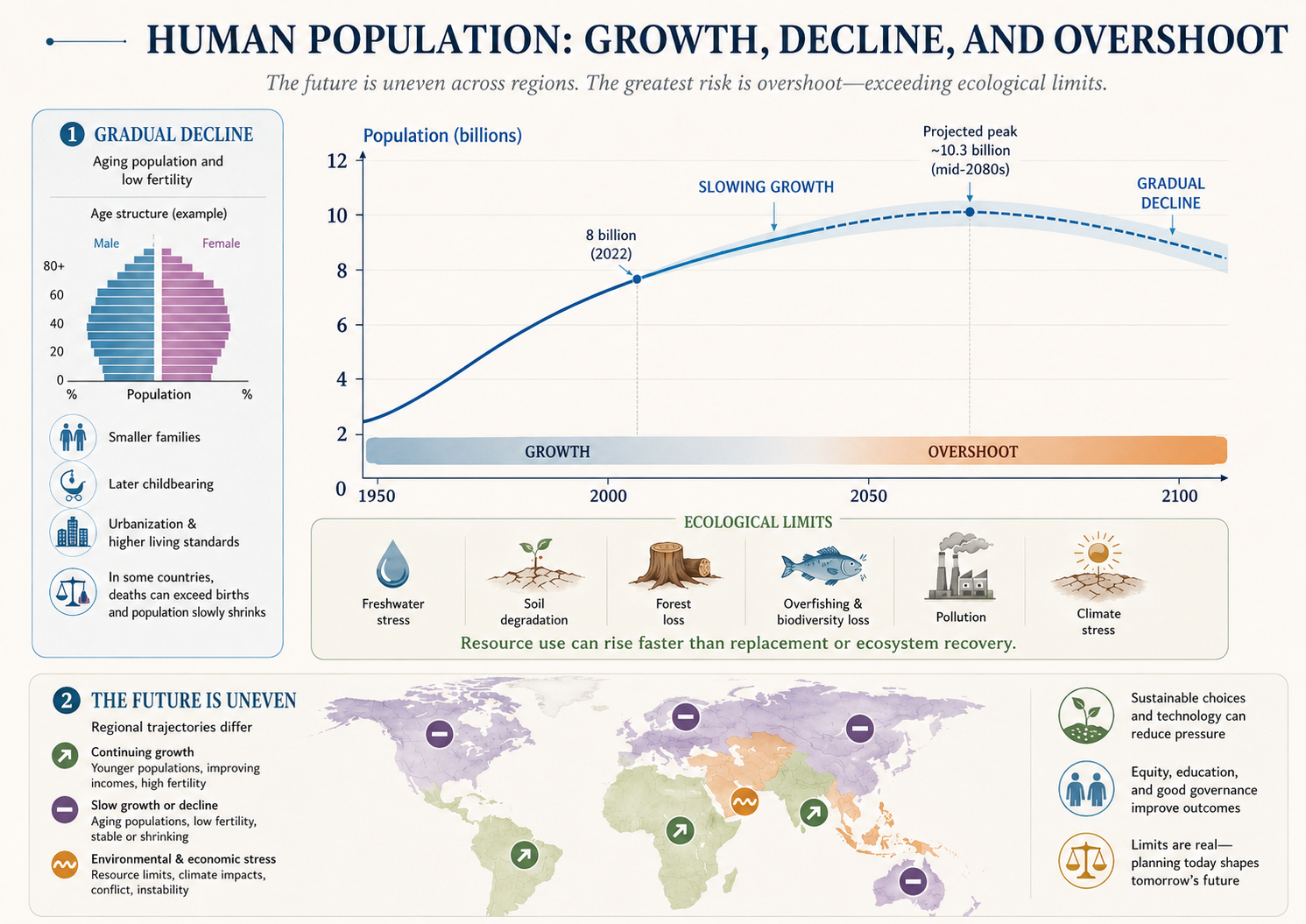
Figure 25. Predicted Human Population Growth, Decline, and Environmental Consequences. The human population is still growing, but current projections suggest growth will slow, peak around the mid-2080s, and then decline slightly by 2100. Future population change will likely vary by region, while environmental consequences will depend on both the number of people and the level of resource consumption.